Long-Distance Running Routes ’ Flat Equivalent Distances from Race

Results and Elevation Proﬁles

Dimitri de Smet

, Michel Verleysen

, Marc Francaux

and Laure nt Baijot

ICTEAM, UCLouvain, Louvain-la-Neuve, Belgium

IoNS, UCLouvain, Louvain-la-Neuve, Belgium

Formyﬁt, Enghien, Belgium

Keywords:

Equivalent Distance, Endurance, Race Times, Running, Collaborative Filtering, GPS Track, Elevation,

Gradient, Ascent.

Abstract:

Running routes’ elevation proﬁles affect their runnability and therefore athletes’ average speeds: route dis-

tances alone are not sufﬁcient to predict or evaluate running times. This is an issue for race preparation, race

strategy, performance comparison and runner workload planning anytime the ground is sloping. This paper

proposes a methodology to establish route equivalent distances expressed as a function of their elevation pro-

ﬁles. The same expression can be used to compute gradient adjusted speeds either for athlete pacing during

races or to analyze their performances afterward. The approach is ﬁrst based on race results and addresses the

problem of attendees’ level disparities by evaluating races and athletes at the same time using a race perfor-

mance model. Subsequently, this paper use polynomial and piecewise linear regressions on the instant slope

along the routes to express equivalent distances. They match previous studies with constant slopes and extend

to the case of varying slopes.

1 INTRODUCTION

Race distances alon e are not sufﬁcient to evaluate

athlete race times. For instance, an athlete who runs

a marathon distance in 3:30’ could be a well prepa-

red casual runner if it happened to be at the Berlin’s

Marathon (known to be particu la rly ﬂat) or he could

be a world class champion if it was the Pikes Peak

Marathon (known to be one of world’s toughest ma-

rathon). Elevation gra dient, weather conditions, alti-

tude, vegetation, uneven grou nd and ground ﬁrmness

affect a thlete speeds. A ﬂat e quivalent distance, tha t

reﬂects all race characte ristics is useful in many ways:

athletes can prepare races considering realistic race

lengths. It also makes athlete ranking possible even if

they did not attend to the same races (this also requires

a p erformance model). This paper describes a m e tho-

dology that assigns ﬂat equivalent distances to routes

based, ﬁrst, on r a ce times and, the n, on their elevation

proﬁles. The ﬂat equivalent distance is deﬁned as the

distance that would be run , on average, in the same

time if the ground was ﬂat; all other above-mentioned

conditions b eing equal. The methodology is applied

on endurance races ranging from 8 to 159km.

Two paths could be taken to achieve the same

goal: through metabolic m easurements or through

statistics on race results. In the ﬁrst appro ach, ﬂat

equivalent distance can be computed as the distance

that would lead to the same energy expenditure on ﬂat

ground. The relationship between energy expenditu re

and gradient of ascent is established by (Minetti e t al.,

2002) by measuring athletes oxygen uptake on an in-

clined treadm ill. This ﬁrst approach is perfectly ﬁne

to assess workload or to plan weight reduction pro-

gram but might not be accurate in what concerns race

times prediction because it does not target it speciﬁ-

cally. The second approach infers a relationship be-

tween race average speeds and their elevation proﬁle

(Kay, 2012; Scarf, 1998; Scarf, 2007). This paper

follows the second approach and addresses two pro-

blems that previous works do n ot take into account.

The ﬁrst problem is that rac e results ca nnot be ea-

sily c ompared because races are not run by the same

set of athletes. There could be attendee level diffe-

rences that dep e nd on the popularity of the race. For

instance, some local races may fail to attract world

elite runners. On the o ther hand, some very popu lar

races may a ttract a crowd of casual runners. This im-

plies that races results (race recor ds or any race statis-

tics) do n ot necessarily reﬂect its objective runnabi-

Smet, D., Verleysen, M., Francaux, M. and Baijot, L.

Long-Distance Running Routes’ Flat Equivalent Distances from Race Results and Elevation Proﬁles.

DOI: 10.5220/0006937000560062

In Proceedings of the 6th International Congress on Sport Sciences Research and Technology Support (icSPORTS 2018), pages 56-62

ISBN: 978-989-758-325-4

lity. This problem is solved by taking a c ollaborative

ﬁltering app roach, inspired by (de Smet et al., 2017),

that evaluates both athletes and races at the same time.

In this way, equivalent distances approximation can

be computed from a collection o f race results tak ing

the attendees’ level into account.

The second problem is that previous attempts fully

describe race elevation proﬁles by two global metrics

that are either the cumulative elevation g ain

(Scarf,

2007) or the average elevation gradient of non-loop

races (fell running races) that present a relatively co n-

stant gradient (Kay, 2012). This is rarely observed

in practice. In the present p a per, the full elevation

proﬁle is considered; this allows for a more realistic

relationship extraction.

To estab lish the desired relationship between ﬂat

equivalent distances and route elevation proﬁles, one

need to possess races’ equivalent distances for which

the elevation proﬁles are kn own. For this purpose,

races equivalent distances are, ﬁrst, established using

race results. This step is referred to as collaborative

ﬁltering (Section 3) . Then, taking elevation proﬁle

data as inputs, a regression mod el that reproduces the

obtained race equivalent distances is built (Sectio n 4).

These two steps are validated by assessing how equi-

valent distances improve race time prediction compa-

red to actual distances.

In the following, all equations are expressed using

SI unit system: speeds in [m/s], times in [s] and eleva-

tion gr adient in [m/m]. Other u nits are used in ﬁgures

for convenience.

2 DATA SOURCES

The two steps methodology requires two kind s of

data. In the ﬁrst step (the collaborative ﬁlterin g part),

race results are used to compute ﬂat equivalent distan-

ces for a set of races. In the second step (the ﬂat equi-

valency modelling part), elevation proﬁles are used to

model ﬂat equivalent distances as a function of the in-

stant elevation gradient along the routes.

2.1 Race Results

A set of 228 031 races times was gathered b y parsing

ofﬁcial results of 61 6 Belgian races. Th ey represent

a large variety of endurance r aces that took place in

2014 and 2015. From these results a subset of 179

674 race times (445 races, 7480 athletes) is kept to

obtain a data set presenting properties that allow a co l-

laborative ﬁltering a pproach to operate (as explained

The cumulative elevation gain is the sum of all positive

vertical displacement along the route.

in Section 3.3). Race results are used to com pute ﬂat

equivalent distances that are then put in relation with

race elevation data.

2.2 Elevation Data

Race routes data were collected through measure-

ments made by runners during the races using their

sports watches. Runners uploaded tracks and made

them publicly available to the online community.

Those tracks contain data such as geographic coor-

dinates, timestamps and altitudes. Consumer grade

GPS-based elevations have poor accuracy (Bauer,

2013). In a previous work (de Sm et et al., 2017) route

elevations we re gathered by querying publicly availa-

ble topography data such a s SRTM data (Shuttle Ra-

dar Topography Mission) or Google Maps APIs. They

are both based on radar topography survey made from

space. It is observed that, in su ch databases, the alti-

tudes of the treetops is assigned to route parts that are

covered by trees: this causes artiﬁcial high elevation

gradients on routes that pass under trees.

Fortunately, some high-end sports watches in-

clude barometric altimeter that have good relative

accuracy: the altitude is known with a n additive bias

that would need to be calibrated . The relative accu-

racy is what is of primarily interest, the absolute alti-

tude accuracy being irrelevant to our purpose as our

analysis is based on elevation gradient only. Routes

recorde d with such devices could be found only for

129 races o f our 445. Those 129 races are used to

model our ﬂat equivalent distance model from eleva-

tion data.

Although more tha n two thirds of the races were

not used in the ﬂat equivalency modelling part, they

are still useful in the c ollaborative ﬁltering part be-

cause they help to ch aracterize athletes and there fore

improve the ﬂat equivalent distance estimation of the

129 races that are used in the ﬂat equivalency model-

ling section.

2.3 Instant Elevation Gradient

Elevation proﬁles as they are record e d, even by high-

end devices, are noisy signals that need to be ﬁltere d;

especially b e cause our application requires to take the

gradient: th e derivative of a noisy signal can take ar-

tiﬁcially high amplitudes. A simple way to take the

gradient and smoo thing at the same time is to take the

average altitude on a n-meters distance ahead min us

the average altitude on the same distance behind. The

chosen distance acts then as a smoothing factor. Mo re

formally, if the elevation proﬁle e(x) is re-sampled

every meter, its gradient g(x) at distance x is given

Long-Distance Running Routes’ Flat Equivalent Distances from Race Results and Elevation Proﬁles

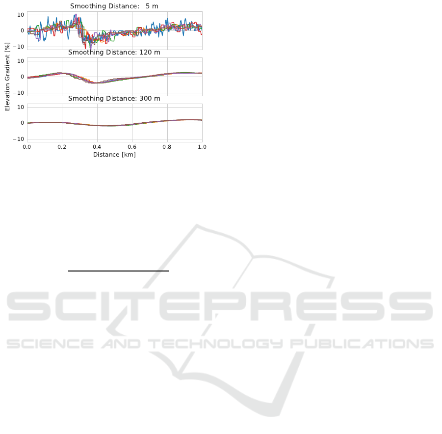
Figure 1: Elevation gradient with different smoothing dis-

tances recorded by 6 different sports watches featuring a

barometric alti meter. On the ﬁrst plot, the elevation gra-

dient is under-smoothed: it shows some details that do not

correlate among measurements. At the opposite, on the last

plot, the elevation gradient is over-smoothed: some details

present in the 6 measurements vanish.

g(x) =

∑

i=x+n

i=x+1

e(x) −

∑

i=x−1

i=x−n

e(x)

, (1)

with n being the smoothing distance in meter. Smoo-

thing reduces the measurement no ise but it also redu-

ces fast changing details of the real gradient. The re-

fore, choosing the smoothing distance n results in a

trade-off that is solved by analyzing its effect on se-

veral track measur ements of the same routes rec orded

by different runner devices. As independence of the

measurement can be assumed, if the ﬁltering distance

is too small, the rando m noise is different on each of

the measuremen t making them less correlated. At the

opposite, a too large smoothing distance makes disap-

pear some details that are present on all the measure-

ment traces. The smoothing problem is illustrated in

Figure 1. Smoothing factor of 120 meters is observed

to be a good trade-off: average tracks pairwise corre-

lation reach a plateau and most small scale elevation

details remain visible.

3 COLLABORATIVE F ILTERIN G

The idea of using c ollaborative ﬁltering presented by

(de Smet et al., 2017) is to take beneﬁt of a collec tion

of race times of many athletes on many races to le-

arn enough information about every race an d every

athlete to best explain race results. The basic under-

lying model is that race times are expla ined by a linear

model of the race paces: the race pace p

a,r

of athlete

a on race r is a sum of products of N race par ameters

times N athlete parameters a

a,r

∑

i=1

· r

. (2)

Races and athletes parameters are found by mini-

mizing the quadratic reconstruction error, i. e. the

sum of the square d differences between observed pa-

ces and paces compu te d with Equation (2).

The simplest case is when N = 1 meaning that the

race pac e is equal to a parameter related to the difﬁ-

culty of the race times a parameter rela ted to the level

of the athlete (low values for high levels). In other

words, g iven all the considered races resu lts, the al-

gorithm outputs race an d athlete parameters that allow

race time predic tion and athlete comparison.

This paper presents a new underlying model that

is more physiologically sou nd and that ma kes the ﬂat

equivalent distance appearing explicitly.

3.1 Race Performances Modelling

Running race times are quite well reﬂected by a po-

wer law (Garc´ıa-Manso et al., 2012): if elevation va-

riations are small enough to not affect the race time,

an athlete a is expected to run race r w ith an average

speed s that depends on the distance as

log(s) ≈ α

· log(D

) + α

(3)

with D

being the actual race distance a nd {α

,α

}

two athlete-speciﬁc pa rameters.

Race time t = D

/s can be expressed as a function

of a ﬁctive ﬂat equivalent distance D

log(t) ≈ w

· log(D

) + w

(4)

with {w

} = {1 − α

,−α

}. Flat equivalent dis-

tances are formally deﬁned a s the distan ces that would

be run in the same time if the ground was ﬂat. They

reﬂect a ll parameters that may affect the average race

speed.

3.2 Equivalent Distances Estimation

Athlete pa rameters (w

a,0

a,1

) and race equ ivalent

distances D

eq,r

in Equa tion(4) are unknown but race

times must reﬂect them.

As the number of race re sults is high, athlete par a-

meters and race equivalent d istance can be set so that

the average squared deviation to Equation(4) is mini-

mized on observed race results.

Let log(t

a,r

) be the log race time of athlete a

on race r and log(

a,r

) its approximation. Using

Equation(4), they can be expressed as

log(

a,r

) = w

a,1

· log(D

eq,r

) + w

a,0

≈ log(t

a,r

). (5)

icSPORTS 2018 - 6th International Congress on Sport Sciences Research and Technology Support

The task at hand is now to select race and athlete pa-

rameters such that our predic tion match observed log

race times.

Let Ω be the set of observed (a,r) for which we

have race results t

a,r

. Using the least square error cri-

terion, athlete and race parameters stor e d in vectors

A and R can be selected by solving the optimization

problem

argmin

A,R

∑

(a,r)∈Ω

(log(t

a,r

) − log(

a,r

))

(6)

This prob le m is solved using an alternate least squa-

res algorithm that alternates between two least squa-

res problems: optimization of the athlete parameters

while holding race parameter constant and optimiza-

tion of the race parameter while holding athle te pa-

rameters constant( Jain et a l., 2013). Convergence is

observed after several iterations, typically 15 to 20.

Solution to Equation (6) does not nece ssarily give

eq,r

that correspond to races ﬂat equiva le nt distan-

ces: the optimal solution has one degree of freed om

because athlete parameters w

are allowed to compen-

sate freely race parameters D

eq,r

Therefore, an extra constraint is required. Some

races present virtually no elevation differences, like

for instance, the Berlin Marathon or some races in co-

astal regions. For races with very ﬂat proﬁle, it can

be expressed that their equivalent distance is equal to

their actual distance:

= D

eq,r

(7)

For a set Ω

of selected ﬂat races, the constraint is

met, on average, if:

∑

Ω

∑

Ω

eq,r

(8)

3.3 Data Conditioning

The ab ove mentioned constraint assumes that a

a,1

and

compen sate each other in th e same way for every

pair of (a,r). This is not guara nteed unless races have

several athletes in common. To ensure th at this con -

dition is met. We deﬁne a proximity metric between

two races as the number o f a thletes who attend to both

of them. By computing this metric for all pair of ra-

ces, we get an adjacency graph fr om which commu-

nity detec tion algo rithm can select clusters of densely

connected races. Using the Louvain algorithm pre-

sented by (Blondel et al., 2008), only the largest and

most densely connected cluster is kept. The later con-

tain 445 races.

In addition, every athlete must have enough race

results to be characterized (in other words, to be ab le

to set his w

and w

parameters) even when one or two

race results are kept aside for validation. Therefore,

the collaborative ﬁltering part is applied on athletes

who h ave at le ast 4 race results. This is the case for

7480 of them.

3.4 Validation

The validation of the collaborative ﬁltering part must

assess its ability to a ssign ﬂat equivalent distances to

races. Given the propo sed deﬁnition of the ﬂat equi-

valent distance, its quality can be evaluated with the

accuracy of race time prediction.

For this purpose, 1 perc ent of the r ace results are

kept aside for validation. All race results but this 1

percent are used to ﬁt th e pa rameters of each athlete

in Equation (4) with the equivalent distance provided

by the collaborative ﬁltering part. This corresponds to

a simple linear regression per athlete. The accuracy is

eva luated by computing the error at predicting the 1

percent race times tha t were not used while solving

Equation (6). The process is repeated 100 times to

reduce the variance of the error estimate.

4 FLAT EQUIVALENCY

MODELLING

Having ﬂat equivalent distance approximation s for a

set of known ra ces, a regression model can be built to

obtain ﬂat equ ivalent distances based on their eleva-

tion proﬁles.

Instant elevation gradients for each point on the

race route are computed from the elevation proﬁle as

described in Section 2.3. Let the function F(g) the

distance correction that need to be applied to a given

sloping distance D presenting an elevation gradient g:

= D · F(g). (9)

If the considered distance presents a varying gra-

dient, it can be split in 1-meter sub-section x presen-

ting a gradient g(x). The equivalent distance of the

whole route is then the sum of the contributions of

each meter :

eq,tot

∑

x=0

F(g

(x)

), (10)

F(g) can take various forms. The present paper is

restricted to piecewise linear and polynomial functi-

ons. Section 4.1 presents different models that are

found in the literature. Section 4. 2 show how model

coefﬁcients can be ﬁtted to reproduce ﬂat equivalent

distance computed with the techniq ue that is presen-

ted in the collaborative ﬁltering part.

Long-Distance Running Routes’ Flat Equivalent Distances from Race Results and Elevation Proﬁles

4.1 Models

Naismith-like Model

The ﬁrst rule of thumb, called the Naismith ’s rule, da-

tes from 1892 and is relayed, among others, by (Scarf,

2007). Naismith’s rule formulated in terms of equi-

valent distances in the sense of our deﬁnition can be

expressed as

= F(g) =

(

1, if (g < 0)

1 + f

· g, if (g > 0)

(11)

with the f

constant being evaluated to 7.92 by (Scarf,

2007).

Polynomial Models

Other papers present a 4

or 5

order polynomial ex-

pressions that take incre ased spe ed for negative gra-

dients into account. (Minetti et al., 2002) gives a rela-

tion that express the m etabolic energy cost of r unning

by distance unit as a 5

order polynomial of the ele-

vation gradient

. This equation will be compared to

ours although their deﬁnition of eq uivale nt distance in

that c a se would be th e distance that would lead to the

same energy expenditure if it was on ﬂat ground.

(Kay, 2 012) gives a 4

order poly nomial that can

be expressed with a deﬁnition o f ﬂat equivalent dis-

tance that matches ours.

4.2 Model Fitting

As stated earlier model ﬁttin g assigns model parame-

ter of the unknown function F() of Eq uation (10) so

that it best reproduce ﬂat equivalent distance that are

established solving the o ptimization problem ( 6) dis-

cussed in the collabora tive ﬁltering section.

For the Naismith- like model, ﬁtting Equation (11)

requires to set the p a rameter f

. This is done by mini-

mizing the least square error o f the equation by com-

puting, for each races, cumulative elevation g a in.

In previous works, the function F was ﬁtted to

route features using global r oute features e ither by as-

suming a constant gradien t or by taking the cumula-

tive elevation gain. In our case, races present varying

gradient. The general polynomial form can be expres-

sed as

= F(g) = 1 +

i=P

∑

i=1

· g

(12)

metabolic energy cost of running was measured by

quantity of oxygen uptake

with P, the polynomial order. The independent

term is set to 1 because F(g) = 1 for g = 0 : the equi-

valent distance o f a route on ﬂat ground is the distance

itself.

The total equivalent distance (10) can then b e writ-

ten as the sum for each meter x along the route as

eq,tot

∑

x=0

[1 +

i=P

∑

i=1

· g

(x)

], (13)

which can the be re-arranged as

eq,tot

= D +

i=P

∑

i=1

[ f

∑

x=0

(x)

], (14)

allowing to pre-compute the inner sum for each race

route. The P model parameters f

can then be compu-

ted using a simple linear regression .

In the equ ation above the runnability is assumed

to only depend on the elevation g radient. This of

course not completely true in practice. The under-

lying assumption is that all other parameters (like we-

ather c onditions) are independent of the elevation pro-

ﬁle so that they will be averaged out in the regression .

4.3 Validation

Just as for the equiva le nt distances provided by

the collaborative ﬁlterin g, the quality of the equiva -

lent distance computed using gradient-based formula

F(g) is evaluated with the accuracy of race time pre-

dictions. Again, for eac h athlete, parameters w

a,0

and

a,0

in Equation (4) can be set using all race results

for which eq uivale nt distance can b e computed except

1 percent that is kept aside for validation. The error

between validation race results and predicted race re-

sults is computed . The process is also repeated 100

times to reduce the variability of the er ror estimate.

5 RESULTS

This section presents the quality of our ﬂat equivalent

distances as pre dictors fo r athletes’ race times using

the Equation (4). As athletes experien ce high variabi-

lity in their performances (especially casua l runners),

race time predictions can not be highly ac curate: 4 to

6 percents error are observed on average. Neverthe-

less, given our deﬁnition of equivalent distance, the

accuracy o f race time prediction is the best way to as-

sess th e quality of the computed equivalent distances.

The boxplot presented in the Figure 2 shows the re-

lative error at predicting athletes’ race times conside-

ring different e quivalent distances. Mode ls expressed

icSPORTS 2018 - 6th International Congress on Sport Sciences Research and Technology Support

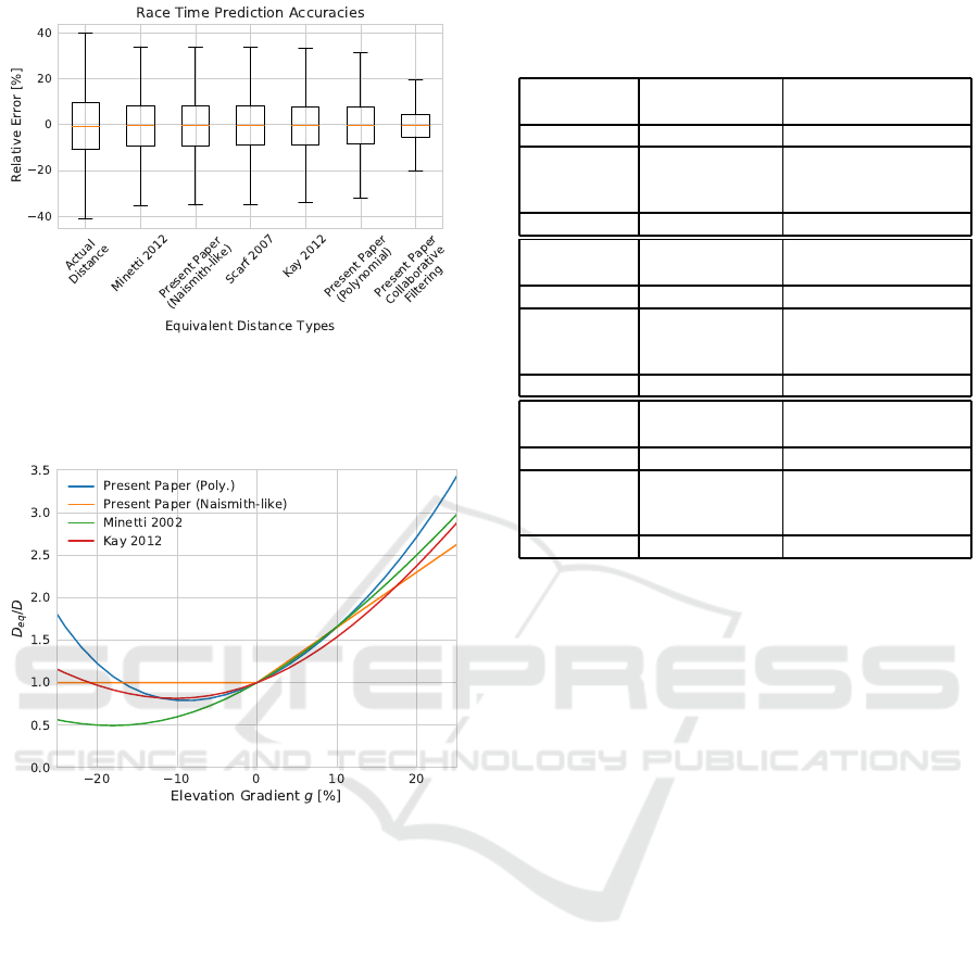
Figure 2: Tukey boxplot representing relative error while

predicting race times with different equivalent distances.

Computing equivalent distances from race results through

collaborative ﬁltering gives the best r esults.

Figure 3: Distance correction based on the elevation gra-

dient.

by Equation s (11) and (12) are evaluate; both with li-

terature coefﬁcients and with co efﬁcients ﬁtted on our

computed equivalent distances. The Table 1 shows

mean relative errors and model param eters.

The Figure 3 shows Naismith’s piecewise linear

model with original coefﬁcient, two polynomial mo-

dels with original coefﬁcients and our best polyn o-

mial ﬁtting (5

order). We can note their relative si-

milarity in th e r a nge that is displayed. As our eleva-

tion proﬁles do not present much grad ie nt outside of

the range [−20%;2 0%], this is also the range of vali-

dity of our model.

6 DISCUSSION

The methodology presented in this paper shows simi-

lar distanc es correction as previous researches with a

novel approa ch that possess some ad vantages.

Table 1: Mean relative errors at predicting race times gi-

ven for different equivalent distances. Actual distances give

7.5%. Collaborative ﬁltering equivalent distances give 4%.

Model Naismith-like 5

order polynomial

(Scarf, 2007) (Minetti et al., 2002)

Equation # (11) (12), P = 5

Coefﬁcients f

= 7.92 { f

1..5

} =

{5.42,12.9,−12.0,

−8.44,43.2}

MRE 6.4 % 6.3 %

Model Naismith-like 4

order polynomial

(present paper) (Kay, 2012)

Equation # (11) (12), P = 4

Coefﬁcients f

= 6.5 { f

1..4

} =

{3.64,17.8,

−3.10,−23.8}

MRE 6.3 % 6.1 %

Model 5

polynomial

(present paper)

Equation # (12), P = 5

Coefﬁcients { f

1..5

} =

{3.90,220,23.6,

6.36,−5.34}

MRE 5.8 %

We obtained ﬂat equivalent distances by ap plying

a collaborative ﬁltering technique on race results.

This technique ta kes beneﬁt of p hysiologically sound

power law to evaluate races’ equivalent distance and

athletes’ level at the same time. By doing so, we ad -

dress the problem of athlete level disparity am ong the

different r a ces.

The obtained ﬂat equ ivalent distances ar e used to

build models that take races elevation proﬁle data as

inputs. Unlike previous works, we apply our distance

correction model to routes with varying gradient.

Results prove that the compu te d equivalent d istan-

ces are more relevant than the ac tual distances as race

time predictors. The best distance correction is the

one that is computed on race results because it cap-

tures all parameters that affect race times (elevation

gradient, weather conditions, ground ﬁrmness, etc.).

Equivalent distances solely based on the routes’ ele-

vation proﬁles give all similar improvements.

Races considered in this paper are all loop race s:

they e nd at the same place as they begin. T herefore,

ﬂat eq uiva lency formulas can not be safely generali-

zed to routes for which it is not the case. This is ob-

vious for Naismith-like formulas: in appearance, the

model only considers decreased speed in uphill secti-

ons; but actually, as it depends on race results, the mo-

del coefﬁcient f

accounts for the fact that there are

necessarily downhill sections were the speed is at le-

ast a little increased. Indeed, a route with only uphill

sections, would be slower than what is predicted by

the N a ism ith-like fo rmulas that are considered here.

Long-Distance Running Routes’ Flat Equivalent Distances from Race Results and Elevation Proﬁles

The polynomial expression that is obtained for

distance adjustment can serve as-is to correct instant

speed on a race route. This could be used, for in-

stance, to optimiz e r ace m anagemen t by providing a

gradient-adjusted target speed along the route.

REFERENCES

Blondel, V. D., Guillaume, J.-L., Lambiotte, R., and Le-

febvre, E. (2008). Fast unfolding of communities in

large networks. Journal of statistical mechanics: the-

ory and experiment, 2008(10):P10008.

de Smet, D., Verleysen, M., and Francaux, M. (2017). Run-

ning race times prediction and runner performances

comparison using a matrix factorization approach. In

5th International Congress on Sport Sciences Rese-

arch and Technology Support.

Garc´ıa-Manso, J., Mart´ın-Gonz´alez, J., Vaamonde, D., and

Da Silva-Grigoletto, M. (2012). The limitations of

scaling laws in the prediction of performance in endu-

rance events. Journal of theoretical biology, 300:324–

329.

Jain, P., Netrapalli, P., and Sanghavi, S. (2013). Low-rank

matrix completion using alternating minimization. In

Proceedings of the forty-ﬁfth annual ACM symposium

on Theory of computing, pages 665–674. ACM.

Kay, A. (2012). Pace and cri tical gradient for hill runners:

an analysis of race records. Journal of Quantitative

Analysis in Sports, 8(4).

Minetti, A. E., Moia, C. , Roi, G. S., Susta, D., and Ferretti,

G. (2002). Energy cost of walking and running at ex-

treme uphill and downhill slopes. Journal of applied

physiology, 93(3):1039–1046.

Scarf, P. (1998). An empirical basis for naismith’s rule.

Mathematics Today-Bulletin of the I nstitute of Mathe-

matics and its Applications, 34(5):149–152.

Scarf, P. (2007). Route choice in mountain navigation,

naismith’s rule, and the equivalence of distance and

climb. Journal of Sports Sciences, 25(6):719–726.

icSPORTS 2018 - 6th International Congress on Sport Sciences Research and Technology Support