On the Effectiveness of Generic Malware Models

Naman Bagga, Fabio Di Troia and Mark Stamp

Department of Computer Science, San Jose State University, San Jose, California, U.S.A.

Keywords:

Malware, Support Vector Machine, k-nearest Neighbor, Chi-squared Test, Random Forest.

Abstract:

Malware detection based on machine learning typically involves training and testing models for each malware

family under consideration. While such an approach can generally achieve good accuracy, it requires many

classiﬁcation steps, resulting in a slow, inefﬁcient, and potentially impractical process. In contrast, classifying

samples as malware or benign based on more generic “families” would be far more efﬁcient. However, ex-

tracting common features from extremely general malware families will likely result in a model that is too

generic to be useful. In this research, we perform controlled experiments to determine the tradeoff between

generality and accuracy—over a variety of machine learning techniques—based on n-gram features.

1 INTRODUCTION

Malware is deﬁned as software that is intended to da-

mage computer systems without the knowledge of the

owner (Norton, 2018). According to Symantec (Sy-

mantec, 2017), more than 357 million new malware

variants were found in 2016. Malware detection is

clearly an important research topic

Signature-based malware detection is effective in

many cases, but fails to detect advanced forms, such

as metamorphic malware. Machine learning techni-

ques including hidden Markov models (HMM), sup-

port vector machines (SVM), k-Nearest Neighbors (k-

NN), and random forests have been used to effectively

detect metamorphic malware, and other challenging

classes of malware (Stamp, 2017). Such models are

often trained using static features, such as opcode se-

quences and byte n-grams.

Previous research has shown that a variety of

techniques based on byte n-grams can achieve rela-

tively high accuracies for the detection problem (Li-

angboonprakong and Sornil, 2013; Reddy and Pujari,

2006; Shabtai et al., 2009; Tabish et al., 2009). Ho-

wever, a recent study based on n-gram analysis rejects

this view and argues that n-grams promote a gross le-

vel of overﬁtting (Raff et al., 2016).

In this research, we consider a somewhat similar

problem as in (Raff et al., 2016), but we take a much

different tack. Our goal here is to perform carefully

controlled experiments that are designed to expose the

relationship between the level of generality of the trai-

ning data and the accuracy of the resulting model. In-

tuitively, we expect that as the training data becomes

more generic, the models will become less accurate,

and our results do indeed support this intuition. We

believe that the results that we provide in this paper

cast the work presented in (Raff et al., 2016) in a much

different light, namely, that the inability to construct a

strong model based on the extremely diverse and ge-

neric data follows immediately from the generality of

the data itself, rather than being an inherent weakness

of a particular feature, such as n-grams.

The remainder of the paper is organized as fol-

lows. In Section 2, we cover relevant background to-

pics, including an overview of selected examples of

related work. This background section also includes a

brief overview of the classiﬁcation techniques used in

this paper, namely, support vector machines, a statisti-

cal χ

score, k-nearest neighbors, and random forests.

Our experiments and results are covered in detail in

Section 3. The paper concludes with Section 4, where

we also discuss future work.

2 BACKGROUND

In this section we discuss selected examples of related

work. Then we also provide a high-level introduction

to each of the various machine learning techniques

employed in the research presented in this paper..

2.1 Related Work

Wong and Stamp (Wong and Stamp, 2006) show that

hidden Markov model (HMM) analysis applied to op-

442

Bagga, N., Troia, F. and Stamp, M.

On the Effectiveness of Generic Malware Models.

DOI: 10.5220/0006921504420450

In Proceedings of the 15th International Joint Conference on e-Business and Telecommunications (ICETE 2018) - Volume 1: DCNET, ICE-B, OPTICS, SIGMAP and WINSYS, pages 442-450

ISBN: 978-989-758-319-3

codes can effectively distinguish some examples of

highly metamorphic malware. The authors trained a

model for each of three different metamorphic mal-

ware families and they were able to successfully dis-

tinguish each family. This malware detection scheme

outperformed commercial anti-virus products. These

results are not particularly surprising, considering that

most commercial products rely on signature based de-

tection methods. This work makes a reasonable case

for the use of opcodes as a feature for malware de-

tection.

Singh et al. (Singh et al., 2016) applied three diffe-

rent techniques to obtain malware scores, namely, an

HMM score, a distance based on principles from sim-

ple substitution cipher cryptanalysis, and an straight-

forward opcode graph score. These three scores were

combined using an SVM to construct a classiﬁer that

was shown to be stronger and more robust than any

of the component scores. This research demonstra-

tes the strength of an SVM, particularly when used to

combine multiple scores into a single classiﬁer.

Reddy and Pujari (Reddy and Pujari, 2006) use

a feature selection method that ranks n-grams based

on frequency and entropy. Their experiments show

that performing a class-wise feature selection impro-

ves the efﬁciency of the models. This process invol-

ves extracting the k most frequent n-grams from the

benign and malware sets and using a union of the two

sets as features. We follow a similar approach in our

n-gram analysis considered here.

Raff et al. (Raff et al., 2016) experimented with

n-grams and elastic-net regularized logistic regres-

sion. These experiments were conducted using a large

dataset containing over 200,000 malware samples.

The detection results obtained from these experiments

were poor and, as mentioned above, the authors claim

that n-grams are not suitable for malware detection.

Unfortunately, the authors’ data was obtained from an

undisclosed “industry partner” and is not available for

independent veriﬁcation of the results.

In this research, we determine the accuracy of n-

gram based malware models as a function of the ge-

nerality of the training data. We see that the more ge-

neric the training dataset, the less distinguishing and

weaker is the resulting model. While this is true in

general, we do observe some differences in various

machine learning techniques, indicating that some ap-

proaches are more robust than others in this respect.

2.2 Classiﬁcation Techniques

In this section we brieﬂy discuss each of the classiﬁ-

cation techniques used in this paper. Speciﬁcally, we

consider support vector machines (SMV), a straight-

forward χ

statistic, k-nearest neighbors, and random

forests. Then in Section 3, each of these techniques

will be used to distinguish between malware and be-

nign samples, based on n-gram frequencies.

2.2.1 Support Vector Machines

SVMs are supervised learning algorithm for binary

classiﬁcation. An SVM is trained on a labeled da-

taset and the resulting model can be used to classify

samples. Conceptually, the main ideas behind SVMs

are the following (Stamp, 2017).

• Separating hyperplane — A hyperplane is con-

structed based on the two classes in the training

data. Ideally, this hyperplane separates the trai-

ning data into its two classes.

• Maximize the margin — The separating hyperplane

is chosen such that the margin between the two

classes of data is maximized. Intuitively, this gi-

ves us the maximum margin for error (relative to

the training data) when using the model to classify

samples.

• Kernel trick — We transform the input data to a

higher dimension feature space using a nonlinear

kernel function. By doing so, we greatly incre-

ase the chance of ﬁnding a separating hyperplane.

The “trick” here is that in spite of the nonlinear

kernel function that we have embedded in the pro-

cess, training and scoring are highly efﬁcient ope-

rations. However, choosing the kernel function is

more art than science. Popular kernel functions

include polynomial learning machines, Gaussian

radial-basis functions (RBF), and two-layer per-

ceptrons.

2.3 Chi-squared Test

The chi-squared test (Plackett, 1983) is a simple and

effective statistical technique that can be applied to

categorical data to determine whether an observed

frequency distribution differs from a speciﬁed fre-

quency distribution. This statistical technique was

ﬁrst described by Pearson (Pearson, 1900) in 1900.

Mathematically, the χ

statistic is essentially a

normalized sum of square deviation between the ex-

pected and observed distributions. This statistic is

computed as

∑

i=1

−E

)

On the Effectiveness of Generic Malware Models

443

where

= cumulative chi-squared statistic

n = number of dimensions or features

= observed value of the i

feature

= expected value of the i

feature

2.4 k-Nearest Neighbors

The k-nearest neighbor (k-NN) algorithm is among

the simplest machine learning algorithms (Stamp,

2017). The k-NN algorithm is a supervised learning

technique and hence requires labeled training data.

In k-NN, we classify a sample based on a majority

vote of the k nearest samples in the training set. Se-

veral variations of k-NN are possible, including weig-

hting the training samples based on their relative fre-

quencies and weighting the “votes” based on their dis-

tance from the sample we are attempting to classify.

One signiﬁcant advantage of k-NN is that it requires

no explicit training phase.

2.5 Random Forests

Random forests are a generalization of a very simple

concept, namely, decision trees (Stamp, 2017). In a

process know as “bagging,” random forests construct

multiple decision trees based on subsets of the trai-

ning data as well as subsets of the available features.

A majority vote of the resulting component decision

trees is used to determine the classiﬁcation of a gi-

ven sample. Bagging reduces the tendency of deci-

sion trees to overﬁt the training data.

3 EXPERIMENTS AND RESULTS

In this section, we discuss the experiments we have

performed and the results obtained. As mentioned

above, the techniques used are SVM, a χ

test, k-NN,

and random forests, all of which are based on n-gram

features. Our primary goal is to carefully analyze the

strength of each of these various models as we add

more malware families into the training set.

3.1 Experimental Design

In all of our experiments, we use the relative frequen-

cies of n-grams as our features, and we conduct expe-

riment based on 2-grams, 3-grams, and 4-grams. The

malware and benign datasets used in our experiments

are discussed in Section 3.2, below.

For all of our n-gram experiments, the feature vec-

tor is based on byte n-gram frequencies. The total

possible number of byte n-grams is 256

= 2

, which

would be challenging to deal with, even for n = 2,

and completely impractical for n > 2. Consequently,

we use a simple feature selection mechanism to re-

duce the size of the feature vector—the approach em-

ployed here is essentially the same as that in (Reddy

and Pujari, 2006). Speciﬁcally, for each n-gram expe-

riment, we select the 10 most frequent n-grams pre-

sent in the malware set and we select the 10 most fre-

quent n-grams present in the benign set, and we form

the union of these two sets, giving us a feature vector

having a maximum length of 20.

For all of our experiments, we use ﬁve-fold cross

validation. That is, the malware dataset is partitioned

into ﬁve equal parts, and each of these parts serves

as the test set in one experiment, with the four remai-

ning parts used for training. In experiments where we

combine multiple malware families, care is taken to

ensure that each of the ﬁve folds (i.e., subsets) con-

tains a balanced number of samples from each family.

Note that cross validation serves to smooth out any

bias in the dataset, while also maximizing the number

of experimental results for the given amount of data

available.

In most of our experiments, we train a model, then

classify samples using the resulting model. To mea-

sure the success of such experiments, we use the con-

cept of balanced accuracy, which is computed as

balanced accuracy =



TP + FN

TN + FP



where

TP = true positives

TN = true negative

FP = false positive

FN = false negative.

Note that the balanced accuracy calculation weig-

hts all classiﬁcation errors the same, regardless of any

imbalance that might exist between the sizes of the

positive and negative sets. This is particularly signiﬁ-

cant in our experiments, since the size of the benign

dataset varies depending on how many malware fa-

milies we combine in one experiment. Because of

this variabillity, a straightforward accuracy calcula-

tion, which is of the form

accuracy =

TP+TN

TP + FN + TN + FP

would, in effect, weight false positive cases less as

more families are considered. Thus, for our experi-

ments, the balanced accuracy provides a more con-

sistent view of the success of our classiﬁers than the

usual (i.e., unbalanced) accuracy calculation.

BASS 2018 - International Workshop on Behavioral Analysis for System Security

444

The χ

experiments discussed below are based

on a scoring function rather than a classiﬁer. Con-

sequently, for these experiments, we computer re-

ceiver operating characteristic (ROC) curves and use

the area under the curve (AUC) as our measure of

success. An ROC curve is constructed by plotting the

true positive rate (TPR) versus the false positive rate

(FPR) as the threshold varies through the range of va-

lues. The TPR is given by

TPR =

TP + FN

while the FPR is computed as

FPR =

FP + TN

The area under the ROC curve (AUC) ranges

from 0 to 1. An AUC of 1.0 indicates perfect sepa-

ration, i.e., there exists a threshold for which no false

positives and no false negatives occur, while an AUC

of 0.5 indicates that the binary classiﬁer is no better

than ﬂipping a fair coin. Also, note that if the AUC

is, say, x < 0.5, then by simply reversing the sense of

the classiﬁer, we obtain an AUC of 1−x > 0.5. In ge-

neral, the AUC gives the probability that a randomly

selected match case scores higher than a randomly se-

lected non-match case (Bradley, 1997; Stamp, 2017).

3.2 Dataset

The following eight families form the malware dataset

used in this research.

Gatak is a trojan that collects information about an

infected computer and sends it to a potential at-

tacker. This trojan hides itself as part of a key

generator application or an update for a legitimate

application (Trojan:Win32/Gatak, 2018).

Kelihos is a family of trojans that send out spam

email with links to installers of malware. This

malware is a botnet that communicates with re-

mote servers to send spam emails and capture sen-

sitive information (Win32/Kelihos, 2018).

Lollipop is an adware program that displays ads as

the user browses the web. This adware can also re-

direct search engine results, monitor a user’s acti-

vity and send such information to an attacker (Ad-

ware:Win32/Lollipop, 2018).

Obfuscator.ACY is a family of viruses that hide

their purpose through various obfuscation techni-

ques. The underlying malware can serve any pur-

pose (VirTool:Win32/Obfuscator.ACY, 2018).

Ramnit is a worm that spreads through infected re-

movable drives. This malware is capable of stea-

ling sensitive information, such as bank credenti-

als (Win32/Ramnit, 2018). Ramnit can give an at-

tacker access to—and control of—an infected ma-

chine.

Winwebsec is a trojan that pretends to be an antivi-

rus product. This malware attempts to convince

the user to pay for its fake antivirus protection by

displaying messages stating that the computer has

been infected (Win32/Winwebsec, 2017).

Zbot (aka Zeus) is a trojan horse that infects sys-

tems by downloading conﬁguration ﬁles or upda-

tes. This ﬁnancial botnet steals conﬁdential infor-

mation, such as online credentials (Trojan.Zbot,

2010).

Zeroaccess is a trojan that makes use of a rootkit

to hide itself. ZeroAccess creates a backdoor on

compromised systems and is capable of down-

loading additional malware (Trojan.Zeroaccess,

2011).

The malware samples used in our experiments

were obtained from the Microsoft Malware Classiﬁ-

cation Challenge (Kaggle, 2015) and the Malicia Pro-

ject (Malicia Project, 2015; Nappa et al., 2013). Table

1 lists the number of samples used from each malware

family. Our representative benign set consists of 300

executables from the System32 folder that were col-

lected from a system running a fresh install of Win-

dows XP.

Table 1: Malware samples per family.

Family Samples

Gatak 1,013

Kelihos 2,942

Lollipop 2,478

Obfuscator.ACY 1,228

Ramnit 1,541

Winwebsec 5,820

Zbot 2,167

Zeroaccess 1,306

total 18,495

For the bigram experiments discussed below, we

consider two cases. First, we use all of the available

malware samples in each family. Then, for a second

set of experiments, we use a balanced malware data-

set, consisting of 1,000 samples from each of the eight

malware families. The balanced experiments provide

more realistic results in cases where a large malware

family (e.g., Winwebsec) is atypical, in the sense of

being either unusually easy or unusually difﬁcult to

On the Effectiveness of Generic Malware Models

445

detect. For our 3-gram and 4-gram experiments, we

use all of the available malware data.

3.3 SVM Experiments

In this section we discuss our SVM experiments ba-

sed on bigram in detail. We then give results for the

equivalent 3-gram and 4-gram experiments.

For each experiment, we determine the relevant

n-grams as discussed in Section 3.1. Once we have

selected the appropriate n-grams, we compute the re-

lative frequencies of each, to yield our feature vectors.

The samples listed in Table 1 were used as our

malware dataset and, as mentioned above, we use a

set of 300 System32 samples as our representative be-

nign samples. An SVM was trained on these datasets

using a radial basis function (RBF) kernel and a soft

margin setting of C = 1.

First, we tested each of the eight malware fami-

lies in Table 1 individually. For each family, we per-

formed one experiment using all available samples

from the family, and we performed another experi-

ment using a selection of 1,000 samples. The balan-

ced accuracies obtained for all of these experiments

are listed in Table 2.

Table 2: SVM balanced accuracy for individual families (bi-

gram models).

Family

Samples per family

all 1,000

Gatak 0.9630 0.9803

Kelihos 0.9983 0.9958

Lollipop 0.8409 0.8757

Obfuscator 0.9199 0.9195

Ramnit 0.8402 0.8619

Winwebsec 0.9712 0.9705

Zbot 0.9614 0.9627

Zeroaccess 0.9793 0.9808

Average 0.9342 0.9434

Next, we train SVMs for each of the





= 28 pairs

of the malware families in our dataset. For example,

one of these experiments consists of combining the

Gatak and Kelihos families into one set, and training

a single SVM to detect members of this combined fa-

mily. As above, we consider both the case where we

use all available samples, and the case where only a

subset of 1,000 samples from each family is conside-

red.

Next, we trained SVMs for all





= 56 combined

sets of three families, and all





= 70 sets of four fa-

milies and so on, up to one super-family that includes

all 8 families. In each case, we compute the average

balanced accuracy over all cases for a given number

of combined families. Table 3 lists these average re-

sults for all possible combinations of the eight mal-

ware families, where the “Families” column refers to

the number of families that were combined.

Table 3: SVM average balanced accuracy (bigram models).

Families

Samples per family

all 1,000

1 0.9342 0.9434

2 0.8806 0.9010

3 0.8402 0.8605

4 0.8081 0.8310

5 0.7827 0.8077

6 0.7603 0.7890

7 0.7384 0.7738

8 0.7265 0.7678

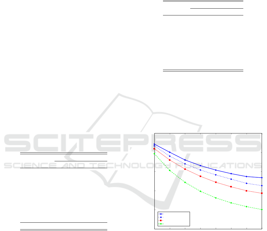
Analogous SVM experiments were conducted ba-

sed on 3-grams and 4-grams, using all of the availa-

ble malware samples. The results of our SVM expe-

riments based on bigrams, 3-grams, and 4-grams are

summarized in the line graphs in Figure 1. Qualita-

tively, we observe that the SVM results for 3-gram

and 4-gram models are similar to those for the bigram

case.

1 2 3 4

5 6

7 8

0.50

0.60

0.70

0.80

0.90

1.00

Number of families

Balanced accuracy

bigram (1000 samples)

bigram (all samples)

3-gram (all samples)

4-gram (all samples)

Figure 1: SVM accuracy vs number of families.

3.4 Chi-squared Experiments

In this section we discuss our experiments and results

using a χ

statistic. The experiments here are essen-

tially the same as those discussed in Section 3.3, ex-

cept that we use a χ

statistic to compute a score, as

opposed to an SVM classiﬁer. Since we have a score

instead of a classiﬁer, we use the area under the ROC

curve as our measure of success, rather than the ba-

lanced accuracy.

BASS 2018 - International Workshop on Behavioral Analysis for System Security

446

For the bigram case, we compute the relative bi-

gram distribution (for the most common bigrams)

over the entire training set. Then to score any sample,

we determine its relative bigram distribution and ﬁnd

the χ

distance from the distribution of the training

set. This is interpreted as a score, where a smaller

value indicates a sample that is closer to the training

set.

When testing each of the eight families individu-

ally, we obtain the AUC values in Table 4. We note

that the range of these results is much greater than the

SVM balanced accuracy discussed above. Here, the

score range from a near-perfect 0.9943 for Winweb-

sec, to a near coin ﬂip of 0.6541 for Lollipop.

Table 4: AUC of χ

score for individual families (bigram

models).

Family

Samples per family

all 1,000

Gatak 0.8784 0.9921

Kelihos 0.9943 0.9930

Lollipop 0.6541 0.6876

Obfuscator 0.8750 0.8712

Ramnit 0.8772 0.8748

Winwebsec 0.9450 0.9384

Zbot 0.8709 0.8646

Zeroaccess 0.9502 0.9472

As with the SVM experiments above, we also con-

sider all combinations of families, and we perform

analogous experiments using 3-gram and 4-grams.

The results of these experiments are summarized in

the form of line graphs in Figure 2.

1 2 3 4

5 6

7 8

0.50

0.60

0.70

0.80

0.90

1.00

Number of families

AUC

bigram (1000 samples)

bigram (all samples)

3-gram (all samples)

4-gram (all samples)

Figure 2: χ

score AUC vs number of families.

The bigram (all samples) and 3-gram cases are vir-

tually indistinguishable in these experiments. Also,

we see that the low score for the Lollipop family drags

down the balanced bigram scores for two families, but

has no appreciable effect on the imbalanced datasets,

as the larger (and easier to detect) families more than

make up for Lollipop.

The results for the χ

score are generally similar to

those for the SVM classiﬁer, in the sense that the more

families we group together, the weaker the results be-

come, on average. However, due to the extremely

poor χ

score for the Lollipop family, the combined

score never falls below that of the weakest individual

score.

3.5 k Nearest Neighbor Experiments

In this section we give our experimental results for

a k-NN classiﬁer, based on n-gram features. Note that

no explicit training is required when using the k-NN

technique—after the n-grams are selected, the (labe-

led) points from the training set form the model. Also,

we need to specify the number of nearest neighbors to

use, i.e., the value of k in k-NN. In all other respects,

the experimental design here is analogous to the SVM

case in Section 3.3, above.

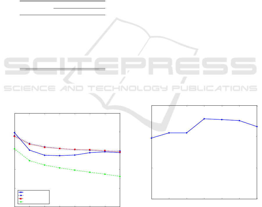
To determine value for k, we performed a set of

experiments on the Gatak family. Speciﬁcally, we tes-

ted each k ∈{2, 3, 4, .. . , 10} and computed the balan-

ced accuracy for each case. Figure 3 depicts the re-

sults of these experiments in the form of a line graph.

Although the differences are relatively small, we see

that k = 5 gives the best results, and hence we have

selected k = 5 for all of our subsequent k-NN experi-

ments.

2 3 4

5 6

7 8

0.90

0.92

0.94

0.96

Balanced accuracy

Figure 3: k-NN results for various values of k.

In Table 5, we give our experimental results—in

the form of the balanced accuracy—for each of the in-

dividual malware families in our dataset. We see that

all families score very high, except Ramnit, which

On the Effectiveness of Generic Malware Models

447

at 86% accuracy (for the “all” case) is signiﬁcantly

below the results obtained for any of the other fami-

lies.

Table 5: k-NN balanced accuracy for individual families

(bigram models).

Family

Samples per family

all 1,000

Gatak 0.9514 1.0000

Kelihos 0.9765 0.9852

Lollipop 0.9334 0.9438

Obfuscator 0.9211 0.9267

Ramnit 0.8632 0.8752

Winwebsec 0.9481 0.9487

Zbot 0.9525 0.9600

Zeroaccess 0.9799 0.9827

We also conducted bigram, 3-gram, and 4-gram

experiments with combined families. The results

obtained for these cases are summarized here in Fi-

gure 4. Qualitatively and quantitatively, our k-NN

results are very similar to those we obtained for the

SVM classiﬁer.

1 2 3 4

5 6

7 8

0.50

0.60

0.70

0.80

0.90

1.00

Number of families

Balanced accuracy

bigram (1000 samples)

bigram (all samples)

3-gram (all samples)

4-gram (all samples)

Figure 4: k-NN balanced accuracy as a function of the num-

ber of families.

3.6 Random Forest Experiments

In this section, we discuss our experiments and results

for random forest classiﬁers. The experimental setup

here is analogous to that used for the SVM and k-NN

experiments considered above. For random forests,

there are many parameters, and we experimented with

a variety of values. For all of the random forest results

presented here, we use the following selection of pa-

rameters.

• The number of trees in each forest is 10.

• Entropy is used to measure the quality of a split.

• We use

√

N features—where N is the total number

of features available in the tree—when determi-

ning the best split. Note that the value of N is

tree-speciﬁc.

• No maximum depth, i.e., nodes are expanded until

all leaves are pure or until all leaves contain less

than 2 samples.

• A minimum of 2 samples is required to split an ex-

isting node.

For each individual family, using random forest

classiﬁers with the parameters listed above, we have

obtained the balanced accuracy results given in Ta-

ble 6. From these results, it is clear that random fo-

rests perform signiﬁcantly better on these individual

families than any of the techniques considered previ-

ously in this paper.

Table 6: Random forest balanced accuracy for individual

families.

Family

Samples per family

all 1,000

Gatak 0.9882 1.0000

Kelihos 0.9982 0.9962

Lollipop 0.9736 0.9750

Obfuscator 0.9505 0.9407

Ramnit 0.9049 0.9079

Winwebsec 0.9897 0.9882

Zbot 0.9894 0.9765

Zeroaccess 0.9887 0.9922

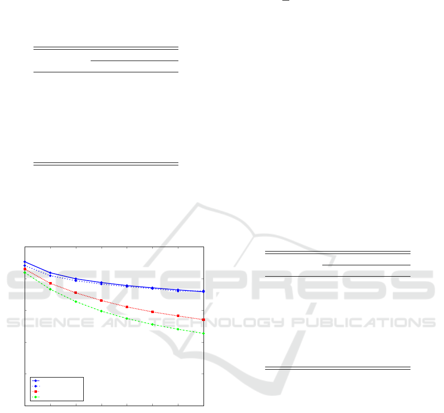
We also conducted bigram, 3-gram, and 4-gram

experiments for random forests. The results for these

cases are summarized in Figure 5. Note that the

two bigram experiments—using all samples versus

using 1,000 samples per family—are virtually indis-

tinguishable in this case.

For our random forest classiﬁers, the average

accuracy drops gradually as we increase the num-

ber of families being modeled. However, the mag-

nitude of the decline is even smaller than we obser-

ved with k-NN. These results indicate that a random

forest is, in some sense, the most robust of the classi-

ﬁers we have considered in this paper. Nevertheless,

the average accuracy of our random forest classiﬁer

does drop to 88% in the bigram case when we con-

struct a model based on all 8 families, which is sig-

niﬁcantly below the lowest accuracy of any of the in-

dividual classiﬁers. Similar statements hold for the

3-gram and 4-gram experiments.

BASS 2018 - International Workshop on Behavioral Analysis for System Security

448

1 2 3 4

5 6

7 8

0.50

0.60

0.70

0.80

0.90

1.00

Number of families

Balanced accuracy

bigram (1000 samples)

bigram (all samples)

3-gram (all samples)

4-gram (all samples)

Figure 5: Random forest balanced accuracy as a function of

the number of families.

3.7 Summary of Results

Figure 6 depicts the variation in average accuracy

with increasing generality of the data for each of the

four techniques considered in this paper. For the χ

experiments, the y-axis represents the area under the

ROC curve (AUC), while for the other three techni-

ques, the y-axis is given in terms of the balanced accu-

racy.

1 2 3 4

5 6

7 8

0.50

0.60

0.70

0.80

0.90

1.00

Number of families

Balanced accuracy/AUC

Random forest

k-NN

SVM

score

Figure 6: Comparison of average accuracy (bigrams using

all samples).

The results in Figure 6 show that a random forest

is the strongest and most robust technique considered

here, followed closely by k-NN, while SVM has the

most signiﬁcant drop off as additional families are in-

cluded. But perhaps the most pertinent observation is

that in every case, a clear trend is apparent—the more

generic the training dataset, the weaker the resulting

model.

4 CONCLUSION

In this paper, we considered four different learning

techniques—SVM, a χ

score, k-NN, and random

forests—and tested the strength of each when faced

with increasingly generic malware “families.” In each

case, we experimented with bigram, 3-gram, and 4-

gram features.

Overall, we found that bigrams gave us the best

results. In addition, the neighborhood based techni-

ques (i.e., random forest and k-NN) proved to be the

strongest, with random forest being the best. In all

cases, we observed that accuracy generally suffers as

the models become more generic.

In our experiments, we considered eight malware

families. Even with this fairly small number of fa-

milies, the effect of an increasingly generic dataset

are readily apparent. Of course, the fewer models we

have to deal with, the better in terms of efﬁciency. Ho-

wever, our results show that we are likely to suffer a

signiﬁcant penalty with respect to classiﬁcation accu-

racy when multiple families are combined into a sin-

gle model, except perhaps in cases where the under-

lying families are closely related. Note that this does

not imply any ﬂaw in the classiﬁcation techniques or

the features used. Indeed, our results show that a sim-

ple bigram feature, for example, can be quite strong

when constructing models within reasonable bounds.

It is also worth noting that the experiments con-

sidered in this paper are, in a sense, a relatively easy

case, as our dataset only has eight well-deﬁned fa-

milies. An extremely large and diverse malware da-

taset is likely to contain a vast number of families,

as well as signiﬁcant numbers of sporadic (i.e., non-

family) malware examples. We would expect any mo-

del trained on such a generic dataset to learn only the

most generic of features. When viewed from this per-

spective, the results given in (Raff et al., 2016) can

be seen to be a natural artifact of the dataset itself,

as opposed to an inherent limitation of the particular

features (i.e., n-grams) under consideration.

For future work, additional features can be consi-

dered. For example, we plan to develop models that

include n-grams, opcodes, and various dynamic fe-

atures, with the goal of analyzing the robustness of

such models in the face of ever more generic data-

sets. While we would certainly expect any model to

deteriorate as the training data becomes more gene-

ric, as a practical matter, anything that can be done

to effectively group more families together—thus re-

On the Effectiveness of Generic Malware Models

449

ducing the number of models required for detection—

while still retaining a usable degree of accuracy would

be a worthy result.

It would also be interesting to study this problem

from the perspective of malware type. That is, can

we achieve greater success if we restrict our attention

to a speciﬁc class of malware, such as botnets, tro-

jans, or worrms, for example? It seems plausible that

there will be more similarity between families that all

belong to the same class than families that span dif-

ferent classes. If so, we would expect to effectively

deal with larger numbers of families within a single

model.

Another basic problem is the need for an extre-

mely large, labeled, and publicly available malware

dataset. While the dataset used here is quite substan-

tial, with 18,495 samples, a dataset with a much larger

number of families (as well as sporadic non-family

malware samples) would be invaluable for research

of the type considered here, as well as for many other

research problems. We are currently in the process of

assembling just such a dataset.

REFERENCES

Adware:Win32/Lollipop (2018). Adware:Win32/Lollipop

threat description. https://www.microsoft.com/en-us/

wdsi/threats/malware-encyclopedia-description?

Name=Adware:Win32/Lollipop.

Bradley, A. P. (1997). The use of the area under the

roc curve in the evaluation of machine learning algo-

rithms. Pattern Recognition, 30(7):1145–1159.

Kaggle (2015). Kaggle: Microsoft malware classiﬁcation

challenge (BIG 2015). https://www.kaggle.com/c/

malware-classiﬁcation/ data.

Liangboonprakong, C. and Sornil, O. (2013). Classiﬁcation

of malware families based on n-grams sequential pat-

tern features. In 2013 IEEE 8th Conference on Indus-

trial Electronics and Applications, ICIEA ’13, pages

777–782.

Malicia Project (2015). Malicia project. http://

malicia-project.com/.

Nappa, A., Raﬁque, M. Z., and Caballero, J. (2013). Dri-

ving in the cloud: An analysis of drive-by download

operations and abuse reporting. In Proceedings of the

10th Conference on Detection of Intrusions and Mal-

ware & Vulnerability Assessment, DIMVA 2013, pa-

ges 1–20.

Norton (2018). Norton Security Center — Malware.

https://us.norton.com/internetsecurity-malware.html.

Pearson, K. (1900). On the criterion that a given system of

deviations from the probable in the case of a correlated

system of variables is such that it can be reasonably

supposed to have arisen from random sampling. The

London, Edinburgh, and Dublin Philosophical Maga-

zine and Journal of Science, 50(302):157–175.

Plackett, R. L. (1983). Karl Pearson and the chi-squared

test. International Statistical Review / Revue Interna-

tionale de Statistique, 51(1):59–72.

Raff, E. et al. (2016). An investigation of byte n-gram fea-

tures for malware classiﬁcation. Journal of Computer

Virology and Hacking Techniques, pages 1–20.

Reddy, D. K. S. and Pujari, A. K. (2006). N-gram analysis

for computer virus detection. Journal in Computer

Virology, 2(3):231–239.

Shabtai, A., Moskovitch, R., Elovici, Y., and Glezer, C.

(2009). Detection of malicious code by applying ma-

chine learning classiﬁers on static features: A state-of-

the-art survey. Information Security Technical Report,

14(1):16 – 29.

Singh, T., Troia, F. D., Visaggio, C. A., Austin, T. H., and

Stamp, M. (2016). Support vector machines and mal-

ware detection. Journal of Computer Virology and

Hacking Techniques, 12(4):203–212.

Stamp, M. (2017). Introduction to Machine Learning with

Applications in Information Security. Chapman and

Hall/CRC, Boca Raton.

Symantec (2017). Symantec internet security threat report.

https://www.symantec.com/content/dam/symantec/

docs/reports/istr-22-2017-en.pdf.

Tabish, S. M., Shaﬁq, M. Z., and Farooq, M. (2009). Mal-

ware detection using statistical analysis of byte-level

ﬁle content. In Proceedings of the ACM SIGKDD

Workshop on CyberSecurity and Intelligence Informa-

tics, CSI-KDD ’09, pages 23–31, New York.

Trojan:Win32/Gatak (2018). Trojan:Win32/Gatak threat

description. https://www.microsoft.com/en-us/wdsi/

threats/malware-encyclopedia-description?

Name=Trojan%3AWin32%2FGatak.

Trojan.Zbot (2010). Trojan.Zbot. http://

www.symantec.com/security response/writeup.jsp?

docid=2010-011016-3514-99.

Trojan.Zeroaccess (2011). Trojan.Zeroaccess. https://

www.symantec.com/security response/writeup.jsp?

docid=2011-071314-0410-99.

VirTool:Win32/Obfuscator.ACY (2018). VirTool:Win32/

Obfuscator.ACY threat description. https://

www.microsoft.com/en-us/wdsi/threats/malware-

encyclopedia-description?Name=VirTool:Win32/

Obfuscator.ACY.

Win32/Kelihos (2018). Win32/Kelihos threat descrip-

tion. https://www.microsoft.com/en-us/wdsi/threats/

malware-encyclopedia-description?Name=Win32

%2fKelihos.

Win32/Ramnit (2018). Win32/Ramnit threat descrip-

tion. https://www.microsoft.com/en-us/wdsi/threats/

malware-encyclopedia-description?Name=Win32/

Ramnit.

Win32/Winwebsec (2017). Win32/Winwebsec. https://

www.microsoft.com/security/portal/threat/encyclopedia/

entry.aspx?Name=Win32%2fWinwebsec.

Wong, W. and Stamp, M. (2006). Hunting for metamorphic

engines. Journal in Computer Virology, 2(3):211–229.

BASS 2018 - International Workshop on Behavioral Analysis for System Security

450