Support Vector Machines for Image Spam Analysis

Aneri Chavda, Katerina Potika, Fabio Di Troia and Mark Stamp

Department of Computer Science, San Jose State University, San Jose, California, U.S.A.

Keywords:

Spam, Image Spam, Support Vector Machine, SVM, Machine Learning.

Abstract:

Email is one of the most common forms of digital communication. Spam is unsolicited bulk email, while

image spam consists of spam text embedded inside an image. Image spam is used as a means to evade text-

based spam ﬁlters, and hence image spam poses a threat to email-based communication. In this research, we

analyze image spam detection using support vector machines (SVMs), which we train on a wide variety of

image features. We use a linear SVM to quantify the relative importance of the features under consideration.

We also develop and analyze a realistic “challenge” dataset that illustrates the limitations of current image

spam detection techniques.

1 INTRODUCTION

Electronic mail or email is one of the most common

forms of digital communication today. Spam can be

deﬁned as unsolicited bulk email. The widespread

use of email makes it an attractive target for spam-

mers. According to a recent report from Syman-

tec (Whitney, 2009), spam now accounts for a stag-

gering 90.4% of all email. Therefore, spam email—

which can include advertisements, malware, phishing

links, adult content, and so on—represents a signiﬁ-

cant threat to the utility of email as a communication

medium.

Initially, spam was virtually always in the form of

text email. Strong classiﬁers have been developed to

ﬁlter such spam, based on content, subject, header,

and so on. For example, Lai and Tsai (Lai and Tsai,

2004) explore four machine learning algorithms that

rely on different parts of an email message. Algo-

rithms including k-nearest neighbors (k-NN), support

vector machines (SVM), and na

ıve Bayes have been

successfully applied to the text-based spam detection

problem.

With the advent of strong text-based classiﬁers,

spammers reacted by developing new techniques—

one such technique is image spam. Spam text em-

bedded inside an image can be an effective method to

evade text-based ﬁlters (Gao et al., 2008).

In its simplest form, image spam contains text that

has been converted to an image. To detect this type of

image spam, optical character recognition (OCR) can

be used to extract the text, which can then be sub-

jected to text based spam detection techniques. As

a reaction to OCR-based detection, spammers em-

ployed obfuscation techniques, which make OCR less

effective (SpamAssasin, 2005).

Instead of detecting image spam based on OCR,

it is possible to consider a more direct approach ba-

sed on properties of the images themselves. In this

research, we consider such an image spam detection

strategy, where image processing techniques are used

in conjunction with machine learning algorithms.

In this research, we improve slightly on the de-

tection results in (Annadatha and Stamp, 2016) by

considering more features. In addition, we have de-

veloped a synthetic image spam dataset, which provi-

des a challenge (but realistic) test case for proposed

image spam detection schemes.

The remainder of this paper is organized as fol-

lows. In Section 2, we give a brief overview of image

spam and related work. In Section 3, we discuss the

features used in our experiments. Section 4 gives

a brief overview of the machine learning techniques

used in our experiments. In Section 5 we discuss the

process that was used to generate our synthetic data-

set and to evaluate its effectiveness. Section 6 pre-

sents out detection results, while Section 7 gives our

conclusions and suggestions for future work.

2 BACKGROUND

In this section, we brieﬂy consider spam detection

techniques. Then we discuss research that is most clo-

Chavda, A., Potika, K., Troia, F. and Stamp, M.

Support Vector Machines for Image Spam Analysis.

DOI: 10.5220/0006921404310441

In Proceedings of the 15th International Joint Conference on e-Business and Telecommunications (ICETE 2018) - Volume 1: DCNET, ICE-B, OPTICS, SIGMAP and WINSYS, pages 431-441

ISBN: 978-989-758-319-3

431

sely related to the work presented in this paper.

2.1 Spam Detection Techniques

From a high level perspective, spam detection techni-

ques can be loosely split into the following two cate-

gories. In practice, these approaches could be used in

various combinations.

• Content based ﬁltering — Content-based schemes

can be used to ﬁlter text spam. These techniques

extract the actual content from within each spam

email and classiﬁers are built based on keywords,

headers, payload, etc. Machine learning techni-

ques have been extensively used for such classi-

ﬁers (Dhanaraj and Karthikeyani, 2013).

• Non-content based ﬁltering — Instead of analy-

zing content directly, we can consider other pro-

perties of email. For example, in the case of image

spam, we can analyze image properties. As men-

tioned above, this is the approach that we follow

in this paper.

2.2 Related Work

Machine learning techniques play a prominent role in

spam detection. For most types of spam, a combina-

tion of image processing and machine learning techni-

ques can yield good results.

Kumaresan et al. (Kumaresan et al., 2015) use se-

veral image features to construct image spam clas-

siﬁers. They use a combination of support vector

machines (SVM) and particle swarm optimization

(PSO). PSO improves the results by iteratively scan-

ning candidate solutions and moving “particles” in the

search space. Due to its computational complexity,

PSO can only deal with a relatively small dataset as

compared to SVM. The authors of (Kumaresan et al.,

2015) claim an accuracy of 90% on the Dredze dataset

(discussed below) using 300 training images and 380

test images.

Another machine learning based approach is con-

sidered by Annadatha et al. (Annadatha and Stamp,

2016), where the feature set consists of 21 image pro-

perties. Each feature is associated with a weight, ba-

sed on how much it contributes to a linear SVM clas-

siﬁcation. Based on these weights, the authors con-

duct various experiments primarily involving feature

selection and feature reduction. These experiments

are conducted on two datasets (Gao et al., 2008; ?)

and, as compared to (Kumaresan et al., 2015), sig-

niﬁcantly more features are used, and the accuracy is

greater on the Dredze dataset. Additionally, an impro-

ved dataset was developed. We have also developed

a challenge dataset, which can be viewed as an im-

provement on the dataset in (Annadatha and Stamp,

2016), in the sense that our image spam is more difﬁ-

cult to distinguish from benign images.

A detection architecture using neural networks is

considered by Soranamageswari et al. (Soranamage-

swari and Meena, 2010), where the authors use back

propagation neural networks (BPNN) for their image

spam detection experiments. They achieve an accu-

racy of 92.82% on the Spam Archive dataset (Fumera

et al., 2006) using color properties of the images.

Chowdhury et al. (Chowdhury et al., 2015) consi-

der metadata features and they present a comparison

of three machine learning algorithms: Na

ıve Bayes,

SVM, and BPNN. The results show that neural net-

works achieve the greater accuracy, at the expense of

increased complexity.

Gao et al. (Gao et al., 2010) analyze a “compre-

hensive” image spam technique that employs both

server-side and client-side detection. Their strategy

is based on a set of 23 image features and relatively

complex detection strategies. In contrast, for the re-

search presented in this paper, we utilize 38 features,

of which 20 overlap with those in (Gao et al., 2010).

We employ a straightforward SVM detector, which al-

lows for a detailed analysis of the relative importance

of the various features.

3 IMAGE FEATURES

Spam images are typically computer generated and

hence they tend to lack color properties and composi-

tion features of a normal “ham” image. For instance,

brightness in ham images tend to vary more than in

spam images.

We use image processing techniques to extract a

total of 38 of features from images. Of these 38 fea-

tures, 21 were considered in (Nixon, 2008). Table 1

gives a brief overview of all the features we have ex-

tracted, where the 21 features in (Nixon, 2008) are

denoted with “ † ”. The features under consideration

can be loosely classiﬁed into the following ﬁve dom-

ains.

• Metadata features — Properties such as image

size, height, width, aspect ratio, compression ra-

tio, and bit depth are the most basic properties of

an image. We consider six metadata features.

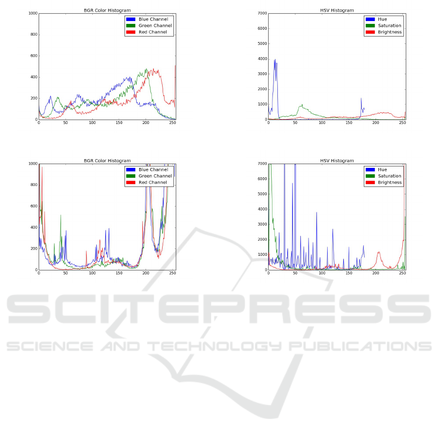
• Color features — Various histograms contain use-

ful information about an image. For example,

color histograms contain information about the

usage of red, green, and blue colors. From Figure

1 we see that the RGB channels of ham and spam

images tend to differ signiﬁcantly.

BASS 2018 - International Workshop on Behavioral Analysis for System Security

432

(a) Ham

(b) Spam

Figure 1: RGB channels of color histogram.

Additional color features are related to hue, sa-

turation, and value (HSV). The hue deﬁnes how

close the color is to red—hue is in the range of 0

to 1, with 0 being red. Saturation is a measure

of the “pureness” of the color, where higher va-

lues of correspond to deeper or richer colors. For

example, white corresponds to 0 saturation. The

value (or intensity) corresponds to brightness. Fi-

gure 2 compares the HSV channels of typical ham

and spam images.

• Texture features — The local binary pattern

(LBP) histogram captures information about the

similarity of each pixel to its neighboring pixels.

The LBP would appear to be a strong feature for

detecting Image spam that is simply text set on a

white background.

• Shape features — We consider a variety of shape

features, including the histogram of oriented gra-

dients (HOG) which describes how the inten-

sity gradient changes in the image. The ed-

ges feature quantiﬁes change in contrast, which

serves to highlight boundaries of features in an

image (Nixon, 2008). Figure 3 shows the Canny

edge ﬁlter results for a spam image and a ham

image. Spam images generally contain text, re-

sulting in an increased number of clear edges as

(a) Ham

(b) Spam

Figure 2: HSV channels of HSV histogram.

compared to ham images. Also, the edges in spam

images tend to be smaller as compared to those in

ham images. We consider the number of edges

and average edge length as two separate features.

• Noise features — We consider two noise featu-

res. The Entropy of Noise is the amount of noise

in an image—typically, spam images have less

noise than ham images. The Signal to Noise Ra-

tio (SNR) is deﬁned to be the ratio of the mean

to the standard deviation in the image histogram,

based on a grayscale version of the image under

consideration.

4 SVM MODELS

In this research, we rely on support vector machine

(SVM) analysis. Neural networks and deep learning

are popular today, and these techniques perform well

in many classiﬁcation tasks. However, when a careful

comparison is done, the differences between deep le-

arning and other machine learning approaches (such

as SVM) is often quite small. For example, in re-

cent research on malware detection based on image

analysis (Yajamanam et al., 2018), it is found that a

Support Vector Machines for Image Spam Analysis

433

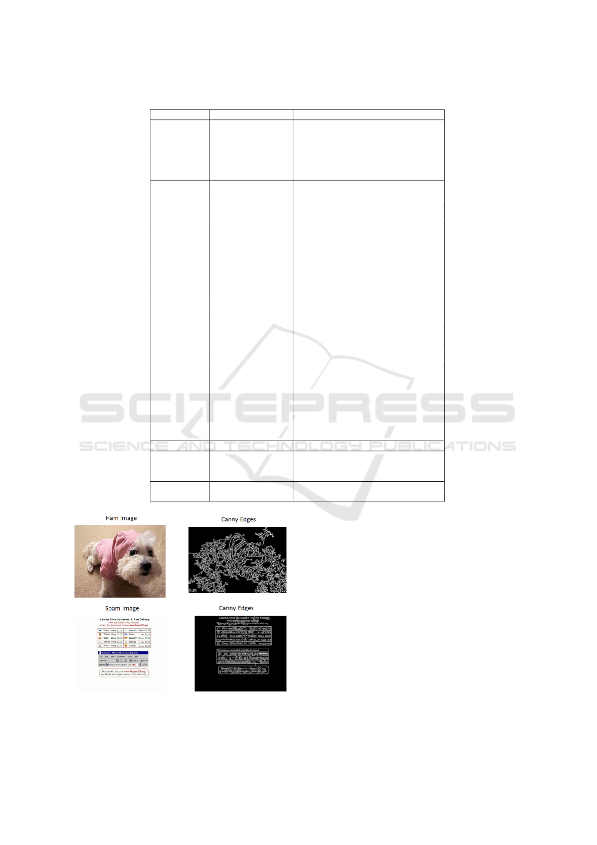
Table 1: Feature set.

Feature Type Feature Description

Metadata

height Height of the image

width Width of image

aspect ratio † Ratio of height and width

compression ratio † How compressed is image

ﬁle size Size on disk

image area Area of image

Color

entr-color † Entropy of color histogram

r-mean † Mean of red histogram

g-mean † Mean of green histogram

b-mean † Mean of blue histogram

r-skew † Skew of red histogram

g-skew † Skew of green histogram

b-skew † Skew of blue histogram

r-var † Variance of red histogram

g-var † Variance of green histogram

b-var † Variance of blue histogram

r-kurt † Kurtosis of red histogram

g-kurt † Kurtosis of green histogram

b-kurt † Kurtosis of blue histogram

entr-hsv Entropy of HSV histogram

h-mean Mean hue of HSV histogram

s-mean Mean saturation of HSV histogram

v-mean Mean brightness of HSV histogram

h-var Variance of hue HSV histogram

s-var Variance of saturation HSV histogram

v-var Variance of brightness HSV histogram

h-skew Skew of hue HSV histogram

s-skew Skew of saturation HSV histogram

v-skew Skew of brightness HSV histogram

h-kurt Kurtosis of hue HSV histogram

s-kurt Kurtosis of saturation HSV histogram

v-kurt Kurtosis of brightness HSV histogram

Texture lbp † Entropy of LBP histogram

Shape

entr-hog † Entropy of HOG

edges † Total number of edges in an image

avg-edge-length † Average edge length

Noise

snr † Signal to noise ratio

entr-noise † Entropy of noise

Figure 3: Canny edges.

simple k-nearest neighbor technique performs nearly

as well as deep learning techniques based on transfer

learning. And an advantage of SVM models is that

they are extremely informative (in particular, linear

SVMs), enabling us to easily determine the contribu-

tion of individual features, perform feature reduction,

quantify interactions between features, and so on. In

contrast, deep learning models tend to be opaque—

essentially, black boxes that produce classiﬁcation re-

sults. Therefore, we believe that SVM is an ideal

technique for the research problems that we consider

in this paper.

SVMs are a class of supervised learning algo-

rithms, generally used for classiﬁcation. SVMs have

been applied to spam detection research in gene-

ral (Lai and Tsai, 2004), and to the image spam de-

tection problem in particular (Annadatha and Stamp,

2016). In this section, we give a brief overview of the

BASS 2018 - International Workshop on Behavioral Analysis for System Security

434

SVM algorithm.

There key concepts that deﬁne the SVM algorithm

are the following (Stamp, 2017).

• Separating hyperplane — In the training phase,

the SVM attempts to divide the labeled input data

into two classes. In the ideal case, the data is line-

arly separable, that is, all data of one class lies on

one side of a separating hyperplane and all data in

the other class falls on the other side of the hyper-

plane.

• Maximize the margin — When constructing an

optimal hyperplane, only a subset of training data

is actually relevant. These special points are

known as support vectors. An optimal hyperplane

is deﬁned as one that maximizes the separation or

margin between the support vectors and the hy-

perplane.

• Work in higher dimensions — In general, the trai-

ning data is not linearly separable in the input

space. By transforming the input data to a hig-

her dimensional feature space, linear separability

can be improved.

• Kernel trick — A kernel function enables us to

map the input space to a higher dimensional fe-

ature space without paying a signiﬁcant cost in

terms of efﬁciency.

4.1 Feature Selection

In a linear SVM, weights are determined for each

input-space feature—the higher the weight, the more

signiﬁcance the SVM classiﬁer places on that feature.

Thus, we can use these weights to rank the features,

and thereby reduce the dimensionality of the problem

without any signiﬁcant loss in accuracy. In fact, we

can sometimes improve the accuracy through feature

reduction, since some features may be so uninforma-

tive as to essentially act as noise.

In this research, we consider recursive feature eli-

mination (RFE), where we initially train a linear SVM

using all available features. Then we eliminate the fe-

ature with the smallest weight and train another linear

SVM on the reduced feature set. We continue to re-

duce the number of features and retrain the SVM until

the desired number of features has been obtained.

4.2 Scoring Metrics

Accuracy is the number of correct classiﬁcations di-

vided by the total number of classiﬁcations, that is,

accuracy =

true positive + true negative

total number of samples

In our detection experiments, we use accuracy as one

quantiﬁable measure of the success (or lack thereof)

of our proposed techniques.

Given the results of any binary classiﬁcation ex-

periment, the receiver operating characteristic (ROC)

curve is constructed by plotting the true positive rate

versus the false positive rate as the threshold varies

through the range of values. The area under the ROC

curve (AUC) ranges from 0 to 1. An AUC of 1.0 indi-

cates perfect separation, i.e., there exists a threshold

for which no false positives or false negatives occur.

On the other hand, an AUC of 0.5 indicates that the

binary classiﬁer is no better than ﬂipping a fair coin.

In general, the AUC gives the probability that a rand-

omly selected match case scores higher than a rand-

omly selected non-match case (Bradley, 1997; Stamp,

2017).

5 DATASETS

Two existing publicly available datasets have been

used in this research. In addition, we have developed

a realistic dataset that is designed to provide a chal-

lenging test for any proposed image spam detection

scheme. All of these datasets contain both spam and

ham images. For our datasets 1 and 2, the ham and

spam images come from actual email, while the chal-

lenge dataset includes modiﬁed spam images.

5.1 ISH Dataset

The developers of Image Spam Hunter (Gao et al.,

2008) collected a large sample of image spam and a

similarly large sample of ham images. We refer to

this data as the ISH dataset. After cleaning the data,

920 spam images and 810 ham images from the ISH

dataset were retained for this research. All of these

images are in jpg format.

5.2 Dredze Dataset

Dredze et. al (Dredze et al., 2007) created an image

spam corpus which is publicly available. Here, we

refer to this set as the the Dredze dataset. After cle-

aning the dataset, we retained 1089 spam and 1029

ham images from the Dredze dataset. As with the ISH

dataset, all images are in the jpg format.

5.3 Challenge Dataset

As discussed above, previous research using publicly

available image spam datasets has obtained strong re-

sults. We also obtain very strong results on these da-

Support Vector Machines for Image Spam Analysis

435

tasets. However, it is clear that image spam could be

made much more difﬁcult to detect. Therefore, we

have also generated our own challenge dataset. As

the name suggests, the purpose of this dataset is to

provide a challenge to the detection of more advan-

ced forms of image spam, which are likely to be seen

in the near future.

We apply various image processing techniques to

actual spam images to make the images look more

like a ham image. We used the Dredze dataset for our

spam corpus, and we overlay ham images from the

ISH dataset.

We experimented with various approaches to de-

velop our challenge dataset and ultimately found that

a relatively simple and straightforward technique was

most effective. To generate our spam images, we ex-

tract the content of an existing spam image, then sim-

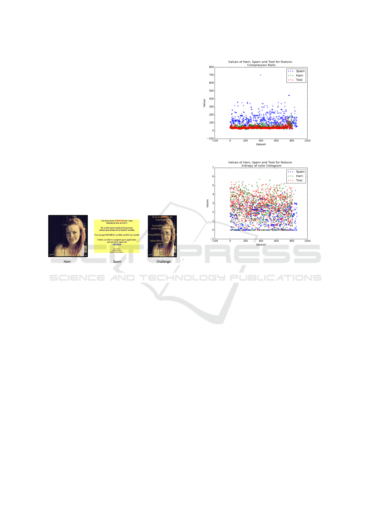
ply overlay it on ham image. Figure 4 shows an ex-

ample of a spam image generated using this approach.

We see that the modiﬁed spam image looks like a ham

image.

Figure 4: Challenge dataset example (second approach).

For the remainder of this paper, “challenge data-

set” refers to the spam images that we have generated

using the method discussed above. A straightforward

SVM detection model was tested on our challenge da-

taset. We found that this SVM gave us a classiﬁca-

tion accuracy of 70%, while more complex techni-

ques could only achieve an accuracy of 79%. Since

our goal is to defeat the detection, this straightforward

approach is better.

Figure 5 shows scatterplots of the compression ra-

tio and color entropy for ham, spam, and our chal-

lenge dataset images. From these scatterplots, it is

clear that the ham and challenge dataset images more

closely align, as compared to those of ham and exis-

ting image spam.

Figure 6 shows differences in SVM weights asso-

ciated with features in the ISH dataset, as compared to

the same feature in the challenge dataset. The majo-

rity of these differences are near 0, indicating that the

SVMs place nearly equal reliance on the correspon-

ding features. This provides further evidence that it

may be difﬁcult to distinguish images in the challenge

dataset from the ham images.

(a) Compression Ratio

(b) Entropy of Color Histogram

Figure 5: Feature value comparison scatterplots.

In the next section, we present and analyze our

main experimental results for ham, spam, and our

challenge datasets. These results are based on SVM

classiﬁcation experiments, and EM clustering experi-

ments.

6 EXPERIMENTS & RESULTS

As previously noted, SVMs have been applied

with success to the text-based spam detection pro-

blem (Dhanaraj and Karthikeyani, 2013). In this

section, we ﬁrst consider SVMs for image spam de-

tection, and we use SVMs for feature reduction. Fi-

nally, we discuss results from clustering experiments.

Below, we conduct experiments on all of the data-

sets discussed above. We obtain strong results on the

ISH and Dredze datasets. As expected, our results are

poor on the challenge dataset, which indicates that it

will present a signiﬁcant challenge for research in this

ﬁeld.

BASS 2018 - International Workshop on Behavioral Analysis for System Security

436

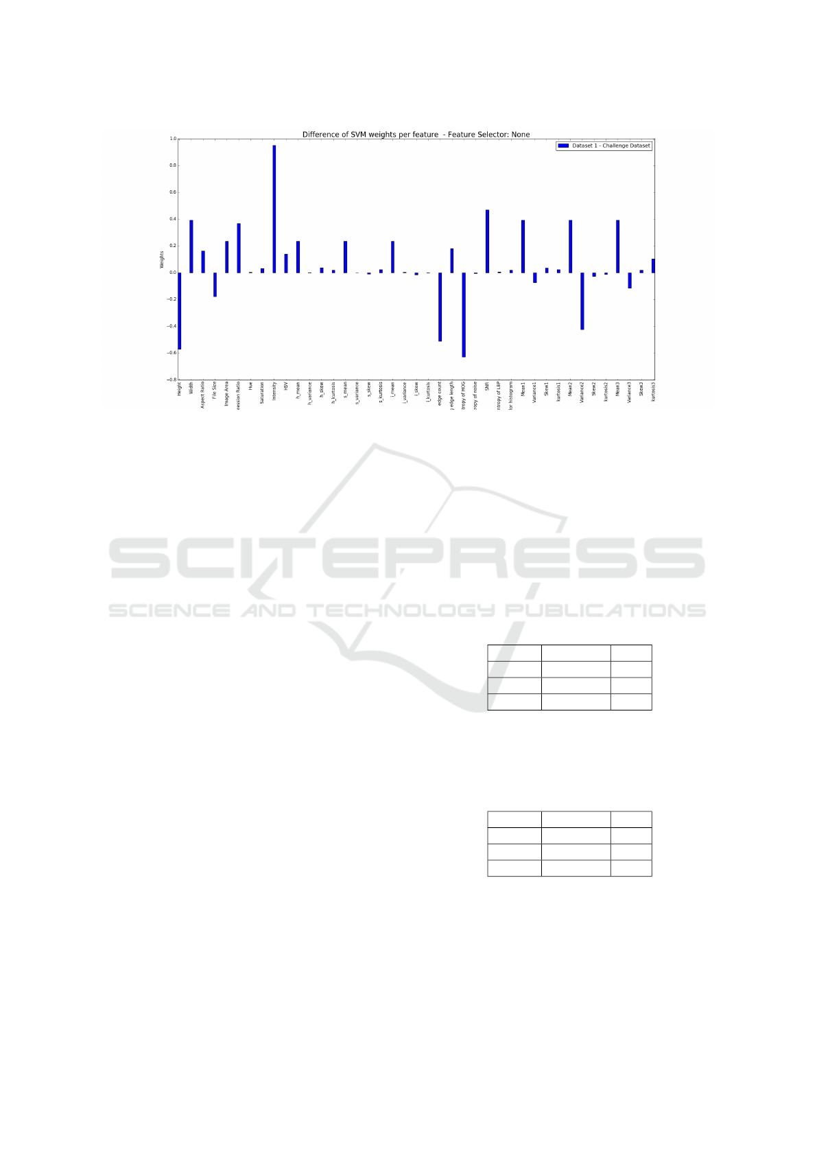
Figure 6: Comparing features of the ISH and challenge datasets.

6.1 SVM Experiments

We have extracted all 38 features from each ham and

spam sample. We train various SVM classiﬁers based

on selected subsets of these features. To measure the

effectiveness of each model, a test set—disjoint from

the training set—is passed to the SVM classiﬁer, with

the accuracy and the area under the ROC curve (AUC)

used to quantify success. In this section, we also ex-

periment with feature reduction to determine optimal

subsets of features.

For each SVM experiment, ﬁve-fold cross valida-

tion is used. That is, for the dataset under conside-

ration, we partition the ham images into ﬁve equal-

sized subsets, which we denote as H

, H

and we do the same for the spam images, and we de-

note these subsets as S

, S

. We then train an

SVM classiﬁer on the labeled datasets H

, H

and S

, S

with H

and S

reserved for tes-

ting the resulting SVM. Then we train an SVM

on H

, H

and S

, S

with H

and S

used for testing, and so on, until each of the ﬁve

pairs (H

, S

) have been used for testing. The results

of all ﬁve “folds” are then combined when determi-

ning the result of the experiment. Cross validation

serves to smooth any bias in the training data, while

also maximizing the number of independent test ca-

ses.

As a ﬁrst attempt to analyze the importance of

each feature, we calculate SVM scores for each fe-

ature individually. That is, for each feature, we trai-

ned and scored using an SVM based only on that one

feature. Figures 7 (a) through 7 (c) give the SVM

results—in the form of AUC statistics—for each indi-

vidual feature, over all three of the datasets. We see

that dataset 1 generally gives the best results while,

as expected, the challenge dataset is the most challen-

ging from the perspective of individual features.

Next, we give results for SVMs where all 38 fe-

atures are used. Again, we consider the ISH dataset,

the Dredze dataset, and our challenge dataset.

Table 2 shows the accuracy and FPR for each of

the three SVM kernels when tested on the ISH dataset.

Here, we achieve the best results for linear kernel.

Table 2: SVM based on 38 features (ISH dataset).

Kernel Accuracy FPR

Linear 0.97 0.05

RBF 0.96 0.06

Poly 0.95 0.07

Table 3 shows the accuracies and FPR for the

same three SVM kernels when tested on the Dredze

dataset. In this case, we achieve equally strong results

for the linear and RBF kernels.

Table 3: SVM based on 38 features (Dredze dataset).

Kernel Accuracy FPR

Linear 0.98 0.01

RBF 0.98 0.01

Poly 0.95 0.09

Although we obtain good results for both the ISH

and Dredze datasets when using the full 38 features,

we obtain slightly better results for the Dredze data-

set. This shows the strength of the SVM, as the results

for individual features in Figure 7 (a), indicate that the

ISH dataset may be the easier case.

Table 4 shows the accuracies and FPR for each of

Support Vector Machines for Image Spam Analysis

437

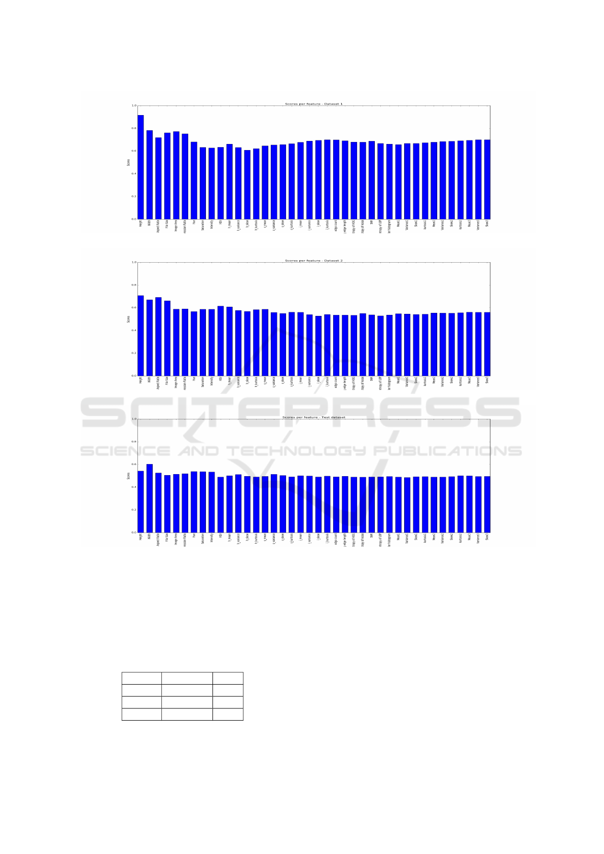
(a) ISH dataset

(b) Dredze dataset

Figure 7: AUC for SVM (individual features).

the three SVM kernels when tested on our challenge

dataset. Again, we achieve the best results using the

linear kernel. As expected, the results are much worse

for this challenge dataset, as compared to the ISH and

Dredze datasets.

Table 4: SVM based on 38 features (challenge dataset).

Kernel Accuracy FPR

Linear 0.68 0.38

RBF 0.64 0.38

Poly 0.54 0.79

6.2 Feature Reduction

Since we have a large number of features, our next

step is to explore techniques to reduce this number

while maintaining (or improving) the overall accu-

racy. Also, reducing the number of features will in-

crease the efﬁciency, which is particularly important

in the detection (or classiﬁcation) phase.

A linear SVM assigns a weight to each feature,

where the weight directly corresponds to the relative

importance of the feature in the SVM classiﬁer. The-

refore, a na

ıve approach to feature reduction is to sim-

BASS 2018 - International Workshop on Behavioral Analysis for System Security

438

ply rank the features based on these weights, elimina-

ting those features with the smallest weights.

However, this is not an ideal strategy as the rela-

tionship between features can change whenever a fe-

ature is eliminated. In this section, we explore recur-

sive feature elimination (RFE), which was discussed

brieﬂy in Section 4.1.

Recall that RFE is a straightforward modiﬁcation

to the na

ıve strategy mentioned in the previous para-

graph. In RFE, we generate a linear SVM and eli-

minate the feature that corresponds to the smallest

weight. Then we generate a new SVM based on this

reduced (by one) feature set and again eliminate the

feature that corresponds to the smallest weight. We

continue this process until some stopping criteria is

met (e.g., we reach the desired number of features, or

the accuracy degrades, or we run out of features).

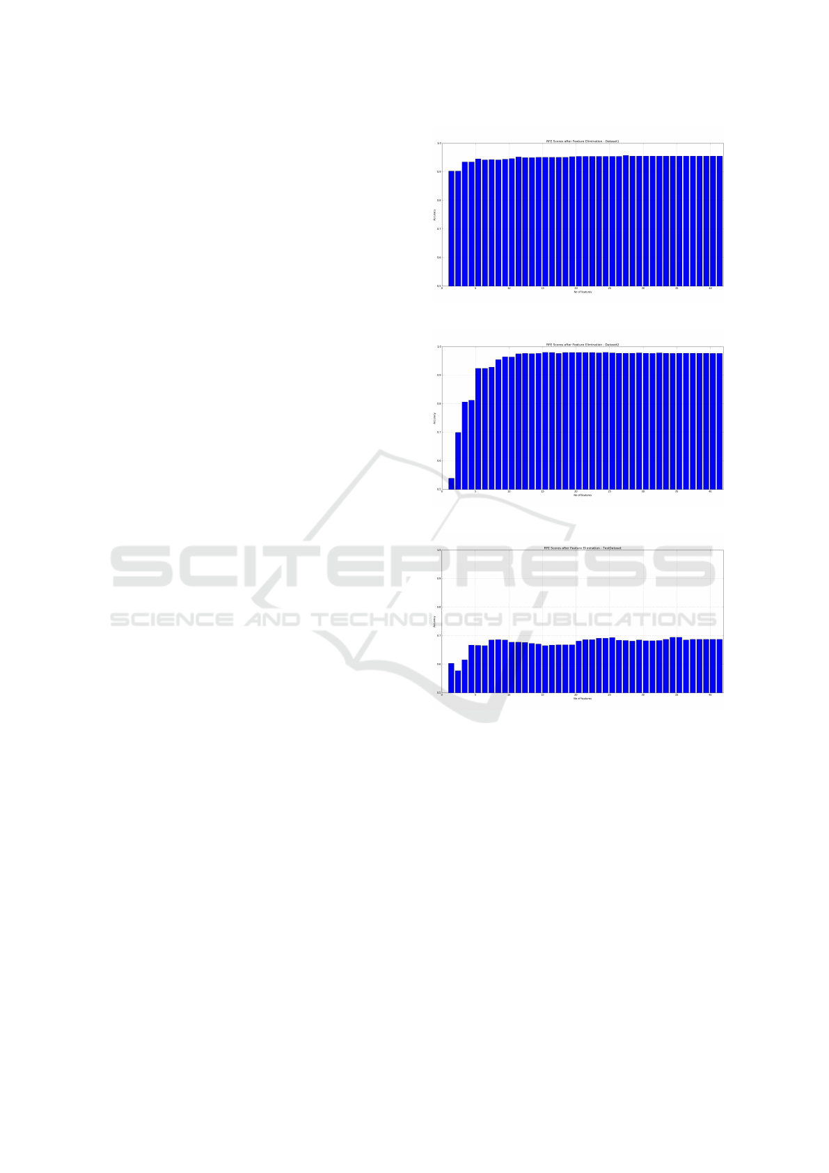
For each dataset, we performed a ranking of all 38

features. Figure 8 (a) shows RFE results for the ISH

dataset. In this case, we achieve a maximum accuracy

of 95.57% when eliminating 13 features.

Figure 8 (b) shows the RFE results for the Dre-

dze dataset. For this particular dataset, the maxi-

mum accuracy is 98.02%, and this occurs when using

only 16 features of the 38 features. In comparison

to the ISH dataset, we require fewer features for the

Dredze dataset and we achieve a higher accuracy.

Finally, Figure 8 (c) gives RFE results for our

challenge dataset. In this case, we achieve a max-

imum accuracy of 69.32% with 26 features which,

again, points to the challenging nature of this dataset.

To summarize, our feature reduction experiments

show that there is redundancy among our 38 features.

This is not surprising, since there are many features

used to measure very similar characteristics. Perhaps

more interesting is the fact that in each case we can

obtain near-optimal results with a small number of fe-

atures. It is also interesting that the accuracy for the

challenge dataset does not exceed 70%.

Next, we present clustering results for our data-

sets. These results provide another perspective on the

inherent challenge of classifying image spam from

each of the sets under consideration.

6.3 EM Clustering

Clustering is an unsupervised machine learning

technique. The essential idea of clustering is to split

the data into sets (or clusters) based on some concept

of distance. The well-known K-means algorithm uses

a simple iterative two-step hill climb which is based

on a direct measure of distance. Expectation maximi-

zation (EM) clustering can be viewed as a generaliza-

tion of K-means, where probability distributions are

(a) ISH dataset

(b) Dredze dataset

Figure 8: RFE results.

used to measure “distance” (Stamp, 2017). Another

way to view the difference between K-means and EM

is that the former generates spherical clusters, whe-

reas the latter allows for more general shapes. Typi-

cally, Gaussian distributions are used in EM cluste-

ring, in which case the resulting clusters can take on

elliptical shapes. In our EM experiments, we employ

Gaussian distributions.

In effect, EM determines the parameters of

unknown probability distributions which are used to

determine the clusters. From a high level perspective,

EM clustering consists of iterating the following two

steps.

1. Expectation Step: Recompute the probabilities for

Support Vector Machines for Image Spam Analysis

439

each datapoint based on the current estimates for

the probability distributions.

2. Maximization Step: Recompute the parameters of

the probability distributions based on the probabi-

lities computed in the expectation step.

Ideally, each cluster will contain only one type of

data. We compute the purity (i.e., uniformity) of the

clusters and use this as our measure of success. The

purity ranges between 0 to 1 with ideal clustering (i.e.,

each cluster contains only one type of data) having a

purity score of 1.0.

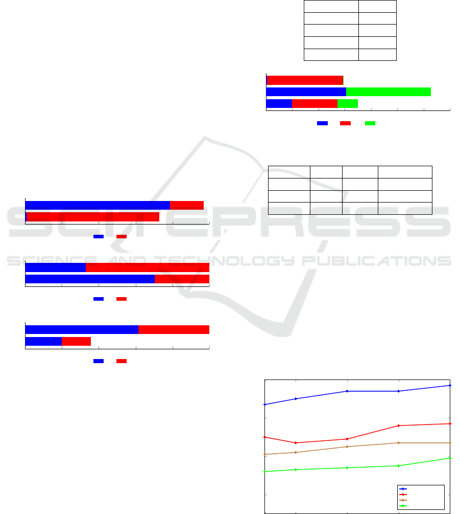
For EM clustering with Gaussian distributions and

two clusters, and using all 38 features, we obtain the

results in Figures 9 (a) through 9 (c). Ideally, one

cluster should contain only ham and the other should

contain only spam. As expected, for the ISH data-

set, the results in Figure 9 (1) appear to be reasona-

bly good, while the results for the challenge dataset

in Figure 9 (c) are very poor. However, the results in

Figure 9 (b) for the Dredze dataset are somewhat sur-

prising. Using an SVM, we can classify the samples

in Dredze dataset with an accuracy comparable to the

ISH dataset, but the clustering results for the Dredze

dataset are much worse than those for the ISH dataset.

0 200 400

600

800 1000

Cluster 2

Cluster 1

Number

Ham

Spam

(a) ISH dataset

0 200 400

600

800 1000

Cluster 2

Cluster 1

Number

Ham

Spam

(b) Dredze dataset

0 200 400

600

800 1000

Cluster 2

Cluster 1

Number

Ham

Spam

Figure 9: EM clustering results.

Table 5 summarizes the purity scores correspon-

ding to the experiments in Figure 9. These scores

conﬁrm the intuitive observations mentioned in the

previous paragraph.

In the next set of clustering experiments, we com-

bined the ISH and challenge datasets and subjected

this combined set to EM clustering. Note that we

have included the ham set, so there are three classes of

data. Using three clusters, we obtain the EM results

in Figure 10, with the corresponding numeric results

summarized in Table 6. Cluster 2, in particular, indi-

cates that a large percentage of the challenge dataset

is indistinguishable from ham. This provides further

strong evidence that the spam images in the challenge

dataset will be difﬁcult to detect using the features

considered in this paper. That is, the challenge dataset

represents a realistic challenge for future research in

this ﬁeld.

Table 5: Clustering results.

Dataset Purity

ISH 0.87

Dredze 0.70

Challenge 0.52

Combined 0.62

0 200 400

600

800 1000 1200 1400

Cluster 3

Cluster 2

Cluster 1

Number

Ham

Spam Challenge

Figure 10: EM with three clusters on combined dataset.

Table 6: Cluster distribution.

Cluster Ham Spam Challenge

1 7 577 4

2 606 0 648

3 197 343 158

We also performed EM clustering with the num-

ber of clusters varying from two to 20. The results of

these experiments are summarized in the form of line

graphs in Figure 11. Intuitively, the purity should in-

crease as we add more clusters—in the extreme, every

sample could be its own cluster, which would yield a

purity of 1.0. Indeed, the purity score does generally

rise as the number of clusters increases. More signi-

ﬁcantly, the gap between each pair of purity scores is

consistent over the range of values tested, indicating

that our results above are not an artifact of the number

of clusters used.

0.40

0.60

0.80

1.00

Clusters

Purity

ISH Dataset

Dredze Dataset

Combined Dataset

Challenge Dataset

Figure 11: Purity scores vs number of clusters.

BASS 2018 - International Workshop on Behavioral Analysis for System Security

440

The results here indicate that even an unsupervi-

sed technique such as EM clustering could be quite

strong against the current crop of image spam. Ho-

wever, if spammers use somewhat more advanced

techniques, it is highly unlikely that the resulting

image spam can be effectively detected using any

combination of the 38 image processing based fea-

tures we have considered in this paper.

7 CONCLUSION

Using samples of real-world ham and spam images,

we showed that machine learning algorithms based on

features extracted by image processing techniques can

be used to construct strong classiﬁers. Our results on

these real-world datasets improves slightly over the

related work in (Annadatha and Stamp, 2016).

We also showed that it is not difﬁcult to generate

much stronger image spam, in the sense that the de-

tection problem is signiﬁcantly more challenging. In

addition, we showed that such improved image spam

cannot be reliably detected using the image proces-

sing based features considered here. These results

improve over the challenge dataset presented in (An-

nadatha and Stamp, 2016), in the sense that the chal-

lenge dataset in this paper is signiﬁcantly more difﬁ-

cult to distinguish from ham, even when using a richer

and more informative feature set. These results indi-

cate that we will likely need new approaches to detect

image spam in the future.

More research is needed to develop and analyze

improved methods for image spam detection. To this

end, we have developed a large image spam challenge

dataset that we will provide to any researchers in this

ﬁeld. By experimenting on this challenge dataset,

it will be possible to directly compare results based

on different proposed detection techniques. Additi-

onal experiments involving this dataset using neural

networks and deep learning would be timely, and it

would be interesting to have such a direct compari-

son between the SVM analysis in this paper, and deep

learning techniques.

REFERENCES

Annadatha, A. and Stamp, M. (2016). Image spam analy-

sis and detection. Journal of Computer Virology and

Hacking Techniques, 23:1–14.

Bradley, A. P. (1997). The use of the area under the

roc curve in the evaluation of machine learning algo-

rithms. Pattern Recognition, 30(7):1145–1159.

Chowdhury, M., Gao, J., and Chowdhury, M. (2015). Image

Spam Classiﬁcation Using Neural Network, pages

622–632. Springer International Publishing, Austra-

lia.

Dhanaraj, S. and Karthikeyani, V. (2013). A study on e-mail

image spam ﬁltering techniques. In 2013 Internatio-

nal Conference on Pattern Recognition, Informatics

and Mobile Engineering, pages 49–55.

Dredze, M., Gevaryahu, R., and Elias-Bachrach, A. (2007).

Learning fast classiﬁers for image spam. In CEAS.

Fumera, G., Pillai, I., and Roli, F. (2006). Spam ﬁltering

based on the analysis of text information embedded

into images. Journal of Machine Learning Research,

7:2699–2720.

Gao, Y., Choudhary, A., and Hua, G. (2010). A comprehen-

sive approach to image spam detection: From server

to client solution. IEEE Transactions on Information

Forensics and Security, 5(4):826–836.

Gao, Y., Yang, M., Zhao, X., Pardo, B., Wu, Y., Pappas,

T. N., and Choudhary, A. (2008). Image spam hun-

ter. In 2008 IEEE International Conference on Acou-

stics, Speech and Signal Processing, pages 1765–

1768. IEEE.

Kumaresan, T., Sanjushree, S., Suhasini, K., and Palani-

samy, C. (2015). Article: Image spam ﬁltering using

support vector machine and particle swarm optimiza-

tion. IJCA Proceedings on National Conference on

Information Processing and Remote Computing, NCI-

PRC 2015(1):17–21. Full text available.

Lai, C.-C. and Tsai, M.-C. (2004). An empirical perfor-

mance comparison of machine learning methods for

spam e-mail categorization. In Fourth Internatio-

nal Conference on Hybrid Intelligent Systems, 2004.

HIS’04., pages 44–48. IEEE.

Nixon, M. (2008). Feature extraction and image proces-

sing. Academic Press.

Soranamageswari, M. and Meena, C. (2010). Statistical fe-

ature extraction for classiﬁcation of image spam using

artiﬁcial neural networks. In 2010 Second Internatio-

nal Conference on Machine Learning and Computing,

pages 101–105.

SpamAssasin (2005). Spamassasin: The apache spamassa-

sin project.

Stamp, M. (2017). Machine Learning with Applications in

Information Security. Chapman and Hall/CRC.

Whitney, L. (2009). Report: Spam now 90 percent of all

e-mail. CNET News, 26.

Yajamanam, S., Selvin, V. R. S., Troia, F. D., and Stamp,

M. (2018). Deep learning versus gist descriptors for

image-based malware classiﬁcation. In Proceedings

of 2nd International Workshop on Formal Methods for

Security Engineering, ForSE ’18.

Support Vector Machines for Image Spam Analysis

441