Improvement of Water Resource Allocation Planning of Inland
Waterways based on Predictive Optimization Approach
Debora C. C. S. Alves, Eric Duviella and Arnaud Doniec
Institut Mines Telecom Lille Douai, URIA, F-59000 Lille, France
Univ. Lille, France
Keywords:
Water-resource Management, Planning, Quadratic Optimization, Predictive Optimization, Large Scale
Systems, Water System.
Abstract:
This paper presents a predictive optimization approach based on a quadratic minimization method to improve
the water resource allocation planning of inland waterways. These networks are large scale systems composed
of several interconnected reaches. Their management consists in keeping the water level of each reach close
to an objective by allocating the available water resource among the network. It is particularly required in the
context of global change where inland waterways should be strongly impacted by flood and drought events.
The designed predictive optimization approach is achieved considering future horizons with the aim to reduce
the impacts of extreme climate events thanks to anticipation of the management actions. A real part of the
inland waterways in the north of France is considered in order to test the designed approach. The obtained
management improvement comparing to water resource allocation planning methods that have been recently
proposed in the literature is highlighted. The influence of the size of the predictive horizon is discussed.
1 INTRODUCTION
The study of the climate change impact on transport
(Tafidis et al., 2017), and more specially on inland
waterways is relatively recent (Koetse and Rietveld,
2009; EnviCom, 2008; IWAC, 2009), with works on
the inland waterways in UK (Arkell and Darch, 2006),
in China (Wang et al., 2007) and on the Rhine (Jon-
keren et al., 2007). The navigation is particularly vul-
nerable to the effects of extreme events, drought and
flood which frequency and intensity are expected hig-
her in close future (Bates et al., 2008; Bo
´
e et al., 2009;
Ducharne et al., 2010). Indeed, the navigation is al-
lowed only when the level of each canal is keeping
inside a navigation rectangle that is defined by two
boundaries around the setpoint: the Normal Naviga-
tion Level (NNL). Hence, an efficient management of
water resource is required. It consists in allocating
the available water and the water in excess (respecti-
vely) among all the waterways during drought peri-
ods and flood periods (respectively). A hierarchical
management strategy has been proposed in (Duviella
et al., 2013) to contribute to this objective. The water
resource allocation planning is achieved in a deter-
ministic way by defining Constraint Satisfaction Pro-
blems (Nouasse et al., 2015; Nouasse et al., 2016b),
with quadratic optimization (Nouasse et al., 2016a),
and with a stochastic view using Markov Decision
Process in (Desquesnes et al., 2016). The quadratic
approach is used considering a part of the real inland
waterways of the north of France in (Duviella et al.,
2018). In (Duviella et al., 2016), a water resource
allocation planning over a future time horizon is pro-
posed to reduce the pumping cost by anticipating the
navigation demand. The proposed approach is based
on a nonlinear programming solver that works by fol-
lowing an iterative process until some stopping crite-
rion is reached. Moreover, it was tested using a fictive
case-study. In this paper, the predictive water resource
allocation planning is based on a quadratic program-
ming solver that yields precise results numerically in a
finite number of steps. This new approach leads to an
improvement of the results that are obtained in (Du-
viella et al., 2018) on the part of the inland waterways
of the north of France. The influence of the size of the
predictive horizon is also discussed.
The paper is organized as follows: the part of the
inland waterways in the north of France that is com-
posed of three reaches is described in Section 2. The
modelling methods that aim at facilitating the imple-
mentation of the allocation planning problem are des-
cribed and exemplified by this case-study. They are
Alves, D., Duviella, E. and Doniec, A.
Improvement of Water Resource Allocation Planning of Inland Waterways based on Predictive Optimization Approach.
DOI: 10.5220/0006918203050312
In Proceedings of the 15th International Conference on Informatics in Control, Automation and Robotics (ICINCO 2018) - Volume 1, pages 305-312
ISBN: 978-989-758-321-6
Copyright © 2018 by SCITEPRESS – Science and Technology Publications, Lda. All rights reserved
305

based on an integrated model and a flow-based net-
work. In section 3, The predictive allocation planning
approach is detailed. Simulation results are provided
in Section 4.
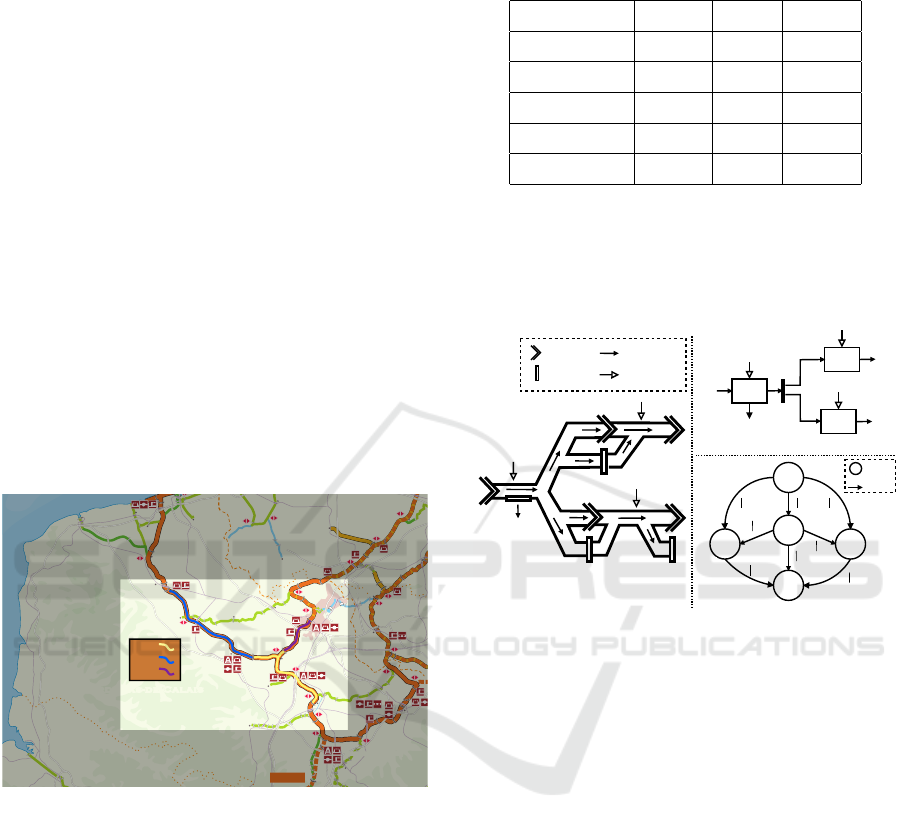
2 CUINCHY-FONTINETTES
SYSTEM
2.1 Description
The studied inland waterways is composed of three
Navigation Reaches (NR) that are linked to the
Cuinchy-Fontinettes reach (see NR
3
in Figure 1); a re-
ach is a part of a canal between at least two locks. The
NR
3
is particularly important for the management of
the waterways in the north of France. In effect, it is an
artificial canal that can be used to dispatch water be-
tween three watersheds. The Cuinchy-Fontinettes re-
ach is also a high water consumer. It is equipped with
a lock downstream that consumes more than 25,000
m
3
at each operation.
A
2
6
A
1
6
A
2
5
A
1
4
A17
Canal Seine-
Nord Europe
LILLE
Arras
Valencien
Armentières
Lens
Douai
Bauvin
Merville
Béthune
Aire-sur-la-Lys
Calais
Gravelines
Watten
Saint-Omer
Bourbourg
Cambrai
Bergues
C.C.
Diksmuide
Ieper
Deinze
Rœselare
Oudenaarde
Kortrij k
Tou rna i
S
c
h
e
l
d
e
L
e
i
e
S
c
a
r
p
e
s
u
p
é
r
i
e
u
r
e
I
J
z
e
r
E
s
c
a
u
t
L
y
s
Aa
L
o
k
a
n
a
a
l
Kanaal Ieper-IJzer
Deûle
C
a
n
a
l
d
e
C
a
l
a
i
s
Kl. Bossuit-
Kortrijk
A
f
l
e
i
d
i
n
g
s
C
a
n
a
l
d
e
B
o
u
r
b
o
u
r
g
C
a
n
a
l
D
u
n
k
e
r
q
u
e
-
E
s
c
a
u
t
C
.
d
e
L
e
n
s
L
y
s
M
i
t
o
y
e
n
n
e
C
a
n
a
l
N
i
m
y
-
H
a
u
t
-
E
s
c
a
u
t
Kl. Rœselare-Leie
Canal
du Nord
S
c
a
r
p
e
i
n
f
é
r
i
e
u
r
e
Canal de
Roubaix
Canal de
l’Espierres
Canal de
l’Espierres
6,5
13
10
14,1
23
13
30,6
16
15,6
14,2
39
48
22
22
8,1
14,3
24,7
10,1
15,1
6,3
28
18,4
33,9
33
14
31,5
11,4
8,5
15,3
30,6
28
5
29,4
17,8
9
37,5
Bruxelles - Capitale
Escautpont
Escautpont
Vaulx
Marquion-Cambrai (SNE)
Marquion-Cambrai (SNE)
Halluin
Prouvy
Rouvignies
Avelgem
Wielsbeke
Arques-
Smetz
Dunkerque-Ouest
Béthune-Beuvry
Guarbecque
Harelbeke
Dourges
Harnes
Sequedin
Santes
Denain
Wallonie
Luxemburg
Saarland
Rheinland-
Pfalz
Nordrhein-
Westfalen
Nord - Pas-de-Cala i s
Picardie
Haute-Normandie
Normandie
Centre
Île-de-France
Bourgogne
Champagne-
Ardenne
Lorraine
Alsace
Vlaanderen
Noord-
Brabant
Limburg
Gelderland
Utrecht
Bruxelles - Capitale
Wallonie
Luxemburg
Saarland
Rheinland-
Pfalz
Nordrhein-
Westfalen
Nord
- Pas-de-Cala i s
Picardie
Haute-Normandie
Normandie
Centre
Île-de-France
Bourgogne
Champagne-
Ardenne
Lorraine
Alsace
Vlaanderen
Zeeland
Zeeland
Noord-
Brabant
Zuid-
Holland
Zuid-
Holland
Limburg
Gelderland
Utrecht
Bruxelles - Capitale
NR1
NR2
NR3
Figure 1: Part of the inland waterways in the north of
France.
The physical characteristics of the three NR are
given in Table 1. The NNL is the water level ob-
jective of each NR that corresponds to the objective
depth. The boundaries, Low Navigation Level (LNL)
and High Navigation Level (HNL) are given in rela-
tive according to the NNL.
2.2 Models
The NR
1
has a distributary configuration (i.e. a dif-
fluence) and supplies the NR
2
and NR
3
thanks to a
gate and a lock in each case. A schematic representa-
tion of the studied network is depicted in Figure 2.a.
The locks are dedicated to the navigation (boat cros-
sing). The gates are used to regulate the water level
Table 1: Dimensions of the NR
i
, level objectives NNL and
navigation limits.
NR NR
1
NR
2
NR
3
Length [km] 56.724 42.3 25.694
Width [m] 41.8 52 45.1
NNL [m] 3.7 4.3 3.3
LNL [m] -0.05 -0.05 -0.05
HNL [m] +0.1 +0.05 +0.05
by controlling the exchanged water volumes between
NR. For a better representation of the type of water
volume exchanges between NR, an integrated model
has been proposed in (Nouasse et al., 2016c). It is
shown for the case study in Figure 2.b.
(a)
Lock
Gate/Dam
NR
2
NR
1
O
S
O
1S
Flow
direction
O
12
NR
3
(c)
NRNR
2
3
O
3S
O
13
d (k)
1
d (k)
2
d (k)
3
Uncontrolled
discharge
NR
1
O
O3
O
O1
O
O2
(b)
Arc
Node
NR
1
V
1
s,c
V
1
e,c
V
1
u
V
1
c
NR
2
V
2
s,c
V
2
e,c
V
2
u
NR
3
V
3
s,c
V
3
e,c
V
3
u
O
2S
Figure 2: (a) Studied network, (b) the integrated volume
model, (c) the flow graph.
The NR can be supplied or emptied by control-
led and uncontrolled water volumes. The controlled
water volumes come from gates and locks. They are
expressed as:
• V
s,c
i
(s: supply, c: controlled) is the controlled vo-
lume that supplies NR
i
from another NR,
• V
e,c
i
(e: empty) is the controlled volume that emp-
ties the NR
i
,
• V
c
i
is the controlled volume from water intakes
that supplies or empties the NR
i
. This volume is
signed. Here it is negative for NR
1
.
The uncontrolled water volumes come from water in-
takes or rain. They are expressed as:
• V
u
i
(u: uncontrolled) is the uncontrolled volume
from natural rivers, rainfall-runoff, Human uses.
These volumes are signed. Here, they are positive
for the three NR.
At each lock operation, an amount of water vo-
lume are exchanged between the upstream NR and
the downstream NR. It is denoted υ
ch
. These water
ICINCO 2018 - 15th International Conference on Informatics in Control, Automation and Robotics
306

volume exchanges depend only to the navigation de-
mand. The gates are controlled to deliver a discharge
inside an operating range. The operating ranges of the
gates are given in Table 2.
Table 2: Characteristics of the NR
i
.
NR NR
1
NR
2
NR
3
Q
c
i
[m
3
/s] [-1; -1] - -
Q
u
i
[m
3
/s] 6.56 0.63 1.2
Q
i
up
[m
3
/s] - [0; 6.4] [0; 30]
Q
i
dw
[m
3
/s] - - [0; 60]
υ
ch
up
.[m
3
] 6.709 3.526 5.904
υ
ch
dw
[m
3
] - 23.000 7.339
In Figure 2.c is depicted the flow-based network
of the case-study. It is built according to the integra-
ted model following the definition and the step given
in (Nouasse et al., 2015). The flow-based network
is composed of a set of ordered nodes (vertices) N
and a set of arcs (directed edges) A. There are nodes
that correspond to the NR and two additional nodes;
a common source vertex O without incoming edges,
a common sink node without outgoing edges, deno-
ted S. The total number of nodes is η = card(N ) + 2.
Hence, the flow-based network G = (N , A) of the sy-
stem is composed of 5 nodes, i.e. η = 5, whose 3
nodes correspond to the three NR.
The arcs represent the possible water exchanges
between the NR, the source, i.e. water volumes that
supply the waterways, and the sink, i.e. water volu-
mes that empty the waterway. The arcs are defined as
a couple a = (i, j), a ∈ R
α
with α = card(A), where i
and j are the origin and destination nodes. At each arc
is associated a flow φ
a
(k) = φ
i j
(k) that represent the
transferred water volumes between nodes i and j at
time k. These flows are bounded by the physical cha-
racteristics of the hydraulic devices. Thus, each flow
has to respect l
i j
(k) ≤ φ
i j
(k) ≤ u
i j
(k), where l
i j
(k)
and u
i j
(k) are the lower and upper bound constraints
respectively.
For the case-study, the flows and their boundary
conditions are given by:























φ
O1
∈ [υ
ch
up
1
· β
O1
(k) + Q
u
1
· T
M
; υ
ch
up
1
· β
O1
(k) + Q
u
1
· T
M
],
φ
O2
∈ [Q
u
2
· T
M
; Q
u
2
· T
M
],
φ
O3
∈ [Q
u
3
· T
M
; Q
u
3
· T
M
],
φ
1S
∈ [Q
c
1
· T
M
; Q
c
1
· T
M
],
φ
2S
∈ [υ
ch
dw
2
· β
2S
(k); υ
ch
dw
2
· β
2S
(k) + Q
2
dw
· T
M
],
φ
3S
∈ [υ
ch
dw
3
· β
3S
(k); υ
ch
dw
3
· β
3S
(k) + Q
c
dw
3
· T
M
],
φ
12
∈ [υ
ch
up
2
· β
12
(k); υ
ch
up
2
· β
12
(k) + Q
c
up
2
· T
M
],
φ
13
∈ [υ
ch
up
3
· β
13
(k); υ
ch
up
3
· β
13
(k) + Q
c
up
3
· T
M
],
(1)
where β
i j
(k) ∈ N is the number of lock operations
of the lock between nodes i and j on a given pe-
riod T
M
, T
M
is expressed in 10
−3
s to obtain volu-
mes in 10
3
· [m
3
], and Q is the upper value of the con-
trolled discharge interval. As an example, the upper
bound capacities for arcs
{
φ
12
, φ
13
, φ
O1
, φ
2S
,φ
3S
}
are
the sum of the maximum available volumes from wa-
ter intakes over T
M
, i.e. V
u
i
= Q
u
i
· T
M
, and volumes
that correspond to the lock operations υ
ch
up
i
· β
i j
(k).
For more details, please refer to the rules defined in
(Nouasse et al., 2015).
2.3 Water Resource Planning Objective
The dynamics of the waterways is modelled by con-
sidering the dynamics of each NR according to the
integrated model. The dynamics of the NR
i
is given
by:
V
i
(k) = V
i
(k − 1) +V
s,c
i
(k) −V
e,c
i
(k) +V
c
i
(k) +V
s,p
i
(k)
−V
e,p
i
(k) +V
u
i
(k),
(2)
where k corresponds to the current period of time and
k − 1 the last one.
This equation can be easily applied to the flow-
based network by considering a relative volume dyn-
amics and by giving a capacity of each node with the
exception of the source and sink nodes. The dynamic
capacity of each node is expressed as:
d
i
(k) = d
i
(k−1)+φ
a
+
(k)−φ
a
−
(k) for i ∈ N −
{
O,S
}
,
(3)
where a
+
is the set of arcs entering the node i, a
−
the set of arcs leaving the node i, and d
i
(k − 1) the
capacity of the node i for the last period.
Then, a relative volume objective that corresponds
to the NNL is introduced. It is denoted D
i
(k), with
i ∈ N −
{
O,S
}
, and such as D
i
(k) = 0. To keep this
objective, the water volume that supplies each node
has to be equal to the water volume that empties it, at
each step time. For real systems, this condition can
not be guaranteed at each step time. Thus, an interval
around the objective D
i
(k) is allowed. It corresponds
to the limits LNL and HNL and leads to d
i
≤ d
i
(k) ≤
¯
d
i
, with d
i
and
¯
d
i
the lower and upper bounds. The
capacity d
i
(k) can be negative or positive.
Even if an interval around the objective D
i
(k) is
allowed, the capacity d
i
(k) has to be closest as pos-
sible to the objective. To this aim, a dynamical cost
function W
i
((D
i
(k) −d
i
(k))
2
), i ∈ N −
{
O,S
}
is as-
sociated to each capacity d
i
(k). This function aims at
penalizing the gap between the current capacity d
i
(k)
and the objective D
i
(k). It is expressed as:
Improvement of Water Resource Allocation Planning of Inland Waterways based on Predictive Optimization Approach
307

W
i
((D
i
− d
i
(k))
2
) =
(
C
max
(d
i
)
2
· (D
i
− d
i
(k))
2
, i f d
i
(k) ≤ 0,
C
max
(d
i
)
2
· (D
i
− d
i
(k))
2
, i f d
i
(k) > 0,
(4)
with C
max
the maximal cost, assuming that d
i
and
d
i
correspond to the lower and upper boundaries re-
spectively.
Moreover, the way to supply or empty one NR has
not the same cost. As example, the volume of water
from natural river may be more expensive than the
volume of water from upstream NR, i.e. water volume
already inside the systems. Thus, a dynamical cost
ω
i j
(k) ∈ R
α
is associated to each arc a. All these
elements are used to define the criteria to optimize.
3 PREDICTIVE ALLOCATION
PLANNING
The optimal water resource allocation consists in sa-
tisfying the objectives of each node, i.e. D
i
(k), by
optimizing the flows Φ(k) in terms of minimal cost.
Two vectors Φ(k) and ∆(k) are introduced to gather
the set of flows φ
i j
(k) and of capacities d
i
(k) at time
k respectively. The optimal sequence of flows Φ
H
is determined by considering a management horizon
H = n × T
M
with n ∈ N and T
M
the management pe-
riod (in hours) to guaranty the objectives D
i
(k) over
the horizon H (Duviella et al., 2016) . The objective
criterion to minimize is:
f
H
(x) =
H
∑
k
"
η
∑
i
W
|
D
i
(k) − d
i
(k)
|
+
α
∑
a
ω
a
(k) × φ
a
(k)
#
,
(5)
with η the number of nodes without nodes O and S,
and α the number of arcs. The initial conditions are
d
i
(k − 1) = 0 for i ∈ [1, η].
The quadratic programming method quadprog in
Matlab is used to minimize f
H
(k) under the equality
constraints defined for each flow and each capacity:
min f
H
(x) such that





L
H
(k) ≤ x
H
(k) ≤ U
H
(k),
A
H
eq
.x(k) = b
H
eq
(k),
A
H
.x(k) ≤ b
H
(k)
(6)
where x
H
(k) is the vector at time k gathering Φ
H
(k)
and ∆
H
(k). The L
H
(k) and U
H
(k) are vectors that
comprises all boundaries of φ
H
(k) and d
H
i
(k) and
have to be computed according to the boundary con-
strains on H. The second condition is the dynamic re-
lation of each node, where b
H
eq
contains the values of
d
i
at the previous period, and A
H
eq
is a vector compo-
sed of 0 or 1 following the structure of the network.
Finally, the last condition is the representations of the
linear coefficients, so A
H
and b
H
are equal to zero.
To calculate the matrix L
H
b
(respectively U
H
b
) is
necessary know the low boundaries (resp. high boun-
daries) on Φ
H
for all the horizon time period. The ma-
trix Ω
H
is composed of the weights of all the arcs for
each step time k ∈ [1,n] of the management horizon
H. These vectors are obtained with the concatenation
of each line of the matrices. For example for H = 3,
if:
L
H
b
=


1 2 3
4 5 6
7 8 9


, (7)
the vector L
H
b
(k) is equal to:
L
H
b
= [1 2 3 4 5 6 7 8 9]. (8)
The vector b
H
(k) is computed of η × n elements
b
H
i,l
(k) with i ∈ [1,η] and l ∈ [1,n]. The index i repre-
sents the node number at the time step l. By conside-
ring only one node over the time horizon H = n × T
M
and the relation (3), it is possible to write the relations
that give the value of the capacity d
1
(l) at each time
step:









d
1
(1) = d
1
(0) + φ
a
+
(1) − φ
a
−
(1)
d
1
(2) = d
1
(1) + φ
a
+
(2) − φ
a
−
(2)
...
d
1
(n − 1) = d
1
(n − 2) + φ
a
+
(n − 1) − φ
a
−
(n − 1)
d
1
(n) = d
1
(n − 1) + φ
a
+
(n) − φ
a
−
(n)
(9)
where d
1
(0) corresponds to the initial capacity of the
node, φ
a
+
(l) (resp. φ
a
−
(l)) are the arcs leaving (resp.
entering) the node 1 at the time step l. Thus, it is
possible to express the value of d
1
(n−1) at time n−1
such:
d
1
(n − 1) = d
1
(0) +
n−1
∑
m=1
[φ
a
+
(m) − φ
a
−
(m)]. (10)
Hence, the components of the vector b
H
(k) can be
computed. Its first elements b
H
i,1
(k), i ∈ [1,η] are equal
to 0. The following elements are computed according
to relations (3) and (11) such as:
b
H
i,l
(k) = b
H
i,1
(k) +
l−1
∑
m=1
[φ
a
+
(m) − φ
a
−
(m)], (11)
with i ∈ [1, η], l ∈ [2,n], where φ
a
+
(m) (resp. φ
a
−
(m))
are the arcs leaving (resp. entering) the node i at the
time step m.
It is also necessary create the matrix Ω
H
that is
composed of the weights of all the arcs for each step
ICINCO 2018 - 15th International Conference on Informatics in Control, Automation and Robotics
308

time k ∈ [1,n]. Then, the algorithm 1 is proposed to
obtain the sequence of optimal flows Φ
H
0
.
That optimization approach leads to the determi-
nation of the optimal sequence of flows on the horizon
H. The proposed approaches are used in next sections
to optimize the water dispatching on a inland naviga-
tion network.
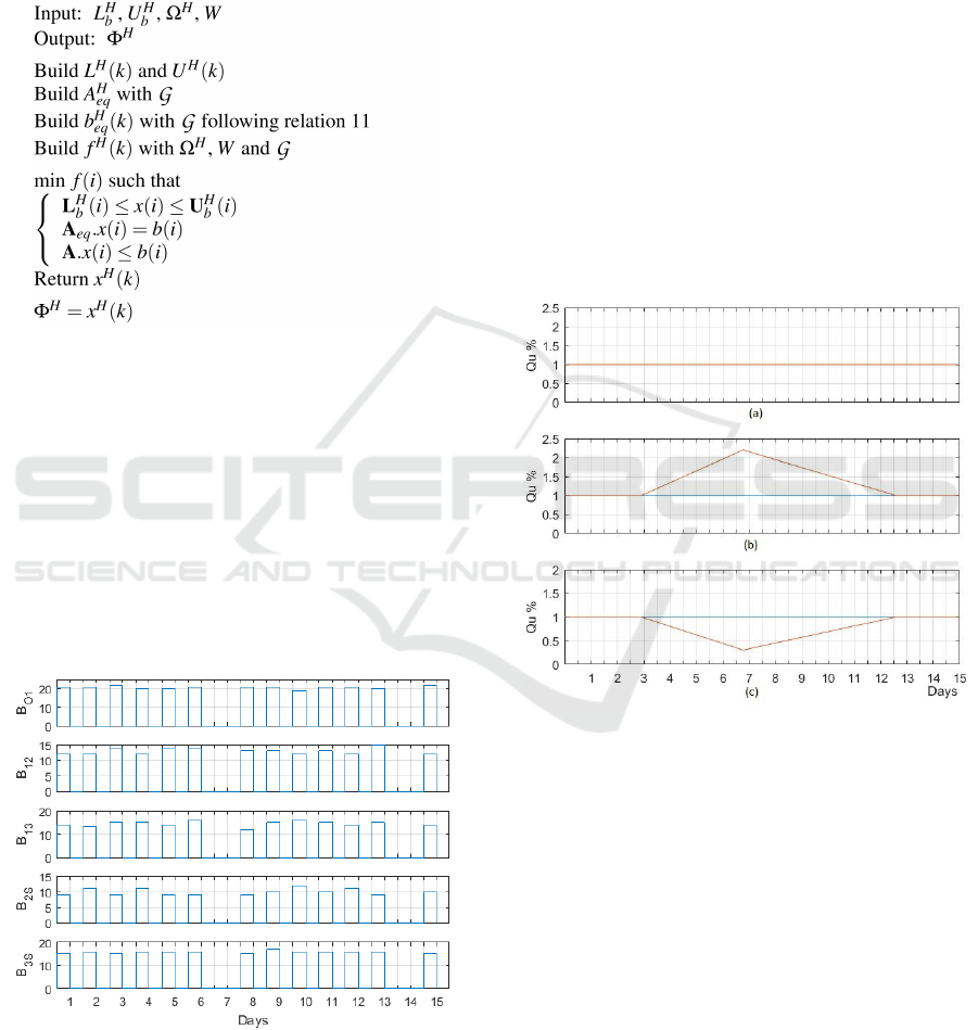
Algorithm 1: Time horizon optimization algorithm.
4 SIMULATION RESULTS
The Cuinchy-Fontinettes system is considered over
two weeks, starting by Monday. The navigation de-
mand is given and the daily lock operations B
i j
are
depicted in Figure 3. The navigation scheduled time
is 14 hours, that means that the remaining 10 hours
(night period) are not allowed the navigation. The na-
vigation is also reduced the 7
th
day that corresponds
to Sunday.
Figure 3: Navigation demand over 15 days.
It is assumed that water volumes that sup-
ply or empty the network from natural rivers
{
φ
O2
, φ
O3
, φ
1S
}
have less priority than the others
{
φ
O1
, φ
12
, φ
13
, φ
2S
, φ
3S
}
. Thus, two different costs
are chosen such as
{
ω
O1
, ω
12
, ω
13
, ω
2S
, ω
3S
}
= 0 and
{
ω
O2
, ω
O3
, ω
1S
}
= 1. In addition, the cost is tune as
C
max
= 2000, a big arbitrary value.
The proposed integrated model of the Cuinchy-
Fontinettes systems has been implemented in Mat-
lab/Simulink. A Matlab function is defined to use the
proposed optimization approach.
Then, three simulated scenarios have been defined
to estimate the impacts of extreme events on the sy-
stem and to study the improvement of the predictive
management strategy. It is supposed that these ex-
treme events have only impacts on uncontrolled dis-
charges from natural rivers. The first scenario is based
on a normal period of navigation. There is no modi-
fication on Q
u
(i) as it is depicted in Figure 4.a. The
second scenario aims at simulating a rainy period with
strong intensity, starting on day 3 and stopping only
on day 12 (see Figure 4.b). The third scenario corre-
sponds to a period of drought (see Figure 4.c).
Figure 4: Climatic event impacts in percentage on uncon-
trolled discharges Q
u
for the three scenarios.
To highlight the improvement providing by the
predictive optimization approach, two different hori-
zons H are considered: H = 1 meaning that the opti-
mization is performed for only the next time (no pre-
diction), and H = 5 days (10 simulation steps).
The simulation results for the first scenario are de-
picted in Figure 5. The red line is the water level. The
blue line corresponds to the HNL, the yellow one to
the LNL. It is shown that the levels in NR
1
and NR
3
remain to the NNL. The most impacted is NR
2
that
can not be emptied during night and during the na-
vigation day-off because no navigation is authorized.
Thus, its level increase during night and Sunday. As
soon as the navigation is allowed, the lock operations
are used to keep its levels to the objective.
When the time horizon (H = 5) is used, there is no
Improvement of Water Resource Allocation Planning of Inland Waterways based on Predictive Optimization Approach
309

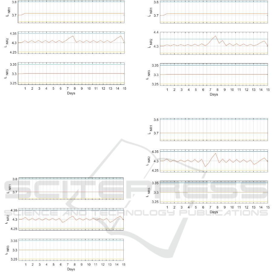
Figure 5: Scenario 1: Levels in (a) NR
1
, (b) NR
2
, (c) NR
3
,
with H = 1.
effect on NR
1
and NR
3
(see Figure 6.a and c). The an-
ticipation on the discharge setpoint on NR
2
leads to a
decrease of the water level during navigation periods
to limit its magnitude during the no navigation peri-
ods. The main improvement can be saw during Sun-
day. Even if the water level of NR
2
oscillates around
the NNL, this strategy is less costly than the previous
simulation in term of global management cost.
Figure 6: Scenario 1: Levels in (a) NR
1
, (b) NR
2
, (c) NR
3
,
with H = 5.
The second scenario highlights the impacts of
strong rain on the Cuinchy-Fontinettes system for
H = 1 (see Figure 7.b). The combination of the
strong rain intensity and the no navigation day leads
to an overflow on NR
2
in days 7 and 8. This rain cre-
ates flood.
The impact of rain is highly reduced when the ho-
rizon H = 5 is used as it is shown for NR
2
in Fi-
gure 8.b. Here again, there is an anticipation in the
setpoint determination that allows to empty more the
NR
2
before the no navigation day. Even if the water
level is close to the HNL on Saturday, the water level
is kept inside the defined boundaries.
Figure 7: Scenario 2: Levels in (a) NR
1
, (b) NR
2
, (c) NR
3
,
with H = 1.
Figure 8: Scenario 2: Levels in (a) NR
1
, (b) NR
2
, (c) NR
3
,
with H = 5.
The drought scenario effects on the Cuinchy-
Fontinettes system are shown in Figure 9 for H = 1.
In this scenario, the most impacted reach is NR
1
. NR
1
is the upstream NR that supplies the two other NR.
Moreover, it has to supply a natural river with a con-
stant control discharge of 1 m
3
/s. Thus, the effect of
the strongest drought periods (day 7) has impacts on
the NR
1
water level in days 8 and 9 (see Figure 9.a).
At the opposite, the water level in NR
2
is close to the
NNL during drought period (see Figure 9.b).
Figure 10 shows that the water resource allocation
planning is improved when H = 5. The water level of
the most impacted NR
1
is kept to the objective NNL.
The water level of NR
2
oscillates around the NNL le-
ading to the optimal global cost of the management
strategy (see Figure 10.b).
These results show that optimizing the water allo-
cation problem by considering the operating horizon
leads to better performance. It remains one question
concerning the size of the prediction horizon. To de-
termine the best value of the prediction horizon, the
ICINCO 2018 - 15th International Conference on Informatics in Control, Automation and Robotics
310

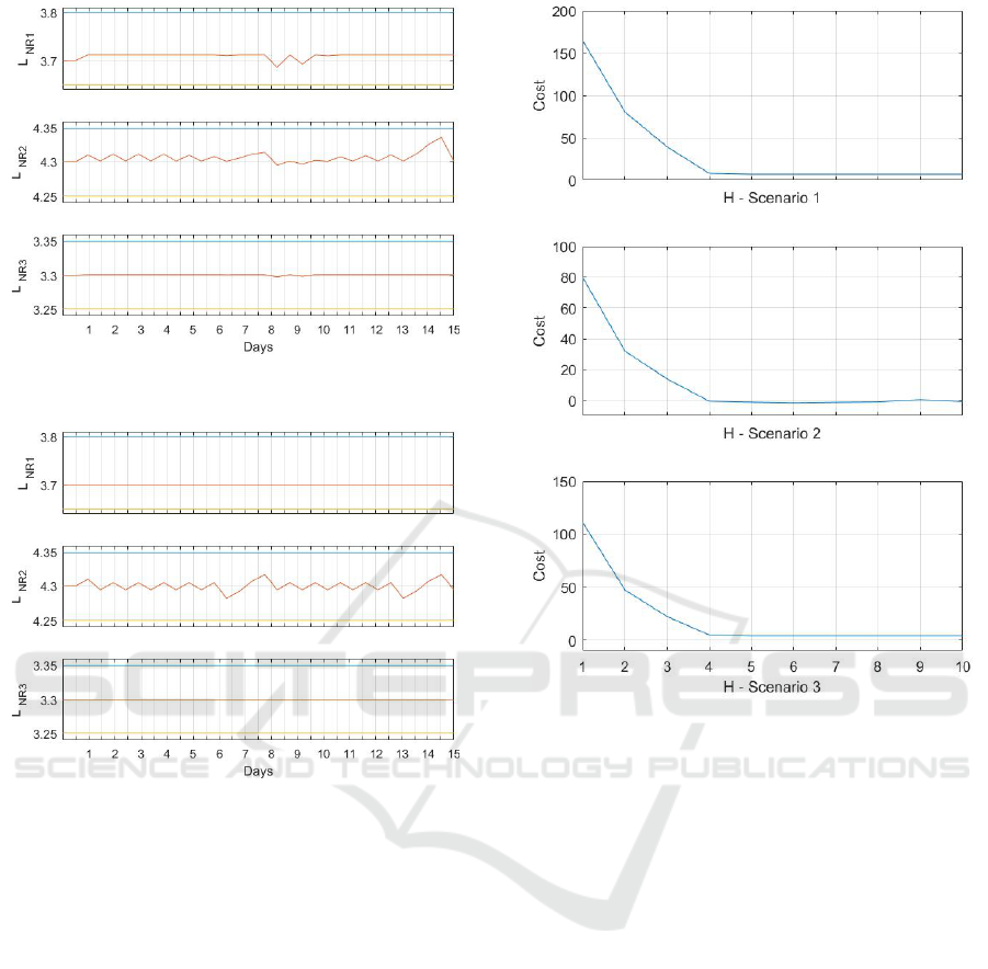
Figure 9: Scenario 3: Levels in (a) NR
1
, (b) NR
2
, (c) NR
3
,
with H = 1.
Figure 10: Scenario 3: Levels in (a) NR
1
, (b) NR
2
, (c) NR
3
,
with H = 5.
three scenarios are considered by increasing the value
of H from 1 to 10. Then, the global cost of the mana-
gement strategy is computed and depicted in Figure
11 for the three scenarios. It is shown that the global
cost decreases between H = 1 to H = 4 and remains
stable for higher values. This is mainly due to the
navigation scheduling of the Cuinchy-Fontinettes sy-
stems and to the fact that the effects of extreme events
are known a priori. That confirms that the considera-
tion of H = 5 was well adapted to the management of
the Cuinchy-Fontinettes systems.
5 CONCLUSIONS
In this paper, a predictive optimization approach ba-
sed on a quadratic minimization method is propo-
sed to improve the water resource allocation plan-
ning of inland waterways. A realistic case study, the
Cuinchy-Fontinettes system is considered to evaluate
Figure 11: Global cost of the management strategy for (a)
scenario 1, (b) scenario 2, (c) scenario 3 according to H.
these improvements by considering drought and rainy
scenarios. The simulation results show that the anti-
cipation of extreme events leads to an efficient mana-
gement of inland waterways. However, even if some
improvements are obtained, uncertainties on the im-
pacts of extreme climate events have not been taken
into account. It will be the main concern of future
works. Moreover, it will be also possible to design a
predictive water allocation planning by considering a
sliding windows.
REFERENCES
Arkell, B. and Darch, G. (2006). Impact of climate change
on london’s transport network. Proceedings of the ICE
- Municipal Engineer, 159:231–237.
Bates, B., Kundzewicz, Z., Wu, S., and Palutikof, J. (2008).
Climate change and water. Technical repport, Inter-
governmental Panel on Climate Change, Geneva.
Bo
´
e, J., Terray, L., Martin, E., and Habetsi, F. (2009). Pro-
jected changes in components of the hydrological cy-
cle in french river basins during the 21st century. Wa-
ter Resources Research, 45.
Improvement of Water Resource Allocation Planning of Inland Waterways based on Predictive Optimization Approach
311

Desquesnes, G., Lozenguez, G., Doniec, A., and Duviella,
E. (2016). Dealing with large mdps, case study of
waterway networks supervision. Advances in Distri-
buted Computing and Artificial Intelligence Journal,
5:71–84.
Ducharne, A., Habets, F., Pag
´
e, C., Sauquet, E., Viennot,
P., D
´
equ
´
e, M., Gascoin, S., Hachour, A., Martin, E.,
Oudin, L., Terray, L., and Thi
´
ery, D. (2010). Cli-
mate change impacts on water resources and hydro-
logical extremes in northern france. XVIII Conference
on Computational Methods in Water Resources, June,
Barcelona, Spain.
Duviella, E., Doniec, A., and Nouasse, H. (2018). Adap-
tive water-resource allocation planning of inland wa-
terways in the context of global change. Journal of
water resources planning and management - Accep-
ted.
Duviella, E., Nouasse, H., Doniec, A., and Chuquet, K.
(2016). Dynamic optimization approaches for re-
source allocation planning in inland navigation net-
works. ETFA2016, Berlin, Germany, September 6-9.
Duviella, E., Rajaoarisoa, L., Blesa, J., and Chuquet, K.
(2013). Adaptive and predictive control architecture
of inland navigation networks in a global change con-
text: application to the cuinchy-fontinettes reach. in
IFAC MIM conference, Saint Petersburg, 19-21 June.
EnviCom (2008). Climate change and navigation - water-
borne transport, ports and waterways: A review of cli-
mate change drivers, impacts, responses and mitiga-
tion. EnviCom - Task Group 3.
IWAC (2009). Climate change mitigation and adaptation.
implications for inland waterways in england and wa-
les. Report.
Jonkeren, O., Rietveld, P., and van Ommeren, J. (2007). Cli-
mate change and inland waterway transport: welfare
effects of low water levels on the river rhine. Journal
of Transport Economics and Policy, 41:387–412.
Koetse, M. J. and Rietveld, P. (2009). The impact of cli-
mate change and weather on transport: An overview
of empirical findings. Transportation Research Part
D: Transport and Environment, 14(3):205 – 221.
Nouasse, H., Doniec, A., Duviella, E., and Chuquet, K.
(2016a). Efficient management of inland navigation
reaches equipped with lift pumps in a climate change
context. 4
th
IAHR Europe Congress, Liege, Belgium
27-29 July.
Nouasse, H., Doniec, A., Lozenguez, G., Duviella, E., Chi-
ron, P., Archim
`
ede, B., and Chuquet, K. (2016b). Con-
straint satisfaction problem based on flow transport
graph to study the resilience of inland navigation net-
works in a climate change context. IFAC Conference
MIM, Troyes, France, 28-30 June.
Nouasse, H., Horv
`
ath, K., Rajaoarisoa, L., Doniec, A., Du-
viella, E., and Chuquet, K. (2016c). Study of global
change impacts on the inland navigation management:
Application on the nord-pas de calais network. Trans-
port Research Arena, Varsovie, Poland.
Nouasse, H., Rajaoarisoa, L., Doniec, A., Chiron, P., Du-
viella, E., Archim
`
ede, B., and Chuquet, K. (2015).
Study of drought impact on inland navigation systems
based on a flow network model. ICAT, Sarajevo, Bos-
nie Herzegovia.
Tafidis, P., Macedo, E., Coelho, M., Niculescu, M., Voicu,
A., Barbu, C., Jianu, N., Pocostales, F., Laranjeira, C.,
and Bandeira, J. (2017). Exploring the impact of ict on
urban mobility in heterogenic regions. Transportation
Research Procedia, 27:309 – 316. 20th EURO Wor-
king Group on Transportation Meeting, EWGT 2017,
4-6 September 2017, Budapest, Hungary.
Wang, S., Kang, S., Zhang, L., and Li, F. (2007). Model-
ling hydrological response to different land-use and
climate change scenarios in the zamu river basin of
northwest china. Hydrological Processes, 22:2502–
2510.
ICINCO 2018 - 15th International Conference on Informatics in Control, Automation and Robotics
312