Using Flexible Time Scale to Explore the Validity of Agent-based

Models of Ecosystem Dynamics: Application to Simulation of a Wild

Rodent Population in a Changing Agricultural Landscape

Jean Le Fur

and Moussa Sall

Institut de Recherche pour le Développement (IRD), Centre de Biologie pour la Gestion des Populations (CBGP),

Campus Baillarguet, CS 30016, F-34988 Montferrier-sur-Lez, France

Dépt. Informatique, Univ.G.Berger/Saint-Louis Sénégal and lab. IRD-BIOPASS, Campus Bel-Air, Dakar, Senegal

Keywords: Agent-based Model, Time Scale, Rodent, Discrete Time Simulation, Sensitivity Analysis.

Abstract: Identifying parameters value is a major issue in model engineering. In discrete time agent-based models,

time step is an important one as it determines the frequency at which agents realize their activity step. This

parameter is commonly defined as a fixed constant during the model design stage. In particular cases, this

may lead to biases as it may be sometimes difficult to determine if agents efficiently realize their activity

step once each 1, 2 seconds, hour or the like. A simulation model of a rodent population has been used to

study the effect of using a flexible time scale on its outcomes. Three types of processes have been

considered as time dependent in the model, environment sensing, movement and life cycle (maturity,

gestation…). A time step sensitivity analysis constitutes the principal result of this study. For the widest

range of time step values, model’s behaviour is unrealistic and bound to algorithms artefacts. A very small

range of time steps leads to simulation of a perennial rodents’ population. Biases bound to variable time step

implementation are discussed. Using flexible time scale approach proved efficient to get insight into the

model’s behaviour and fruitful clues to assess agents’ processes frequency in the actual ecosystem.

1 INTRODUCTION

Agent-based models are recognized as powerful

approaches to formalize ecological processes (White,

2016; Fu and Hao, 2018). This formalism is wide-

spread in social systems modelling (Squazzoni, 2010),

whether animal or specifically human systems, as it

can make emerge organization patterns out of agents’

interaction (Whitley, 2016). As for other models, one

important focus must be put in agent-based models on

calibration of parameters used to describe the

simulated populations (Stanilov, 2011). Indeed,

following Watts (2016), an agent-based model whose

parameters are not conveniently fitted may be useless,

even with a good representation of its agents’ logic.

Several directions are proposed in the literature

to simulate agent-based models with a particular

distinction between discrete time and discrete events

simulation (Buss et al., 2010). Among these

alternatives, discrete time simulations are widely

used (Railsback et al., 2017) as they constitute a

practical and easier to implement approach (Floudas

et al., 2004) to formalize concrete systems, be them

natural (Singh et al, 2018), social (Sauser et al.,

2018) or economical (Ponomarenko et al., 2018). In

discrete time simulations, agents are sequentially

allowed to perform one cycle of activity each given

time step. As a general rule, parameters calibrations

are realized for a fixed time step uniformly

incremented (Al Rowaei et al., 2011). Recent work

on this question put forward the significant impact

that using a fixed time step could have on the

outcomes of such type of models (Buss and Rowaei,

2010, Kuo, 2015). Indeed, one cycle usually implies

agents’ decision processes about their environment

such as perception-deliberation-execution in a PDE

scheme (Ferber and Müller, 1996) or Belief-Desire-

Intention in a BDI scheme (Caillou et al., 2017).

Whatever the scheme however, it is often difficult, if

possible, to determine if one agent has to process the

selected scheme once each second, two seconds,

minute, hour, day or the like.

In this study we are interested in configuring a

classical agent-based model of a rodent population

in the wild. The aim is to evaluate the optimal time

step duration to fulfil the need of the model’s

objective, that is to say, make evolve a perennial

population in a changing landscape. Beyond the

Fur, J. and Sall, M.

Using Flexible Time Scale to Explore the Validity of Agent-based Models of Ecosystem Dynamics: Application to Simulation of a Wild Rodent Population in a Changing Agricultural Landscape.

DOI: 10.5220/0006912702970304

In Proceedings of 8th International Conference on Simulation and Modeling Methodologies, Technologies and Applications (SIMULTECH 2018), pages 297-304

ISBN: 978-989-758-323-0

297

model design with its environment, agents’

behaviour, etc., we designed the model so as it could

be run at various time scales in order to determine

the convenient time step necessary for this purpose

and thereafter use the model accordingly.

The article is first devoted to the presentation of

the model and the approach used to implement a

flexible time scale. The use case is then described

along with the simulation protocol and its associated

time-scale sensitivity analysis. The results section

presents the outcomes of the model for a range of

time steps used. Results and the method used to

formalize time scale changes are then discussed

before concluding on perspectives and possible

improvements.

2 MODEL AND USE CASE

DESCRIPTION

2.1 General Model Overview

The general model used is described in Le Fur et al.

(2017). It is coded in Java using the Repast

Simphony Platform (North et al., 2005). It is a

combination of three connected class hierarchies;

one for substrates at different spatial aggregation

levels, one for genes and genomes that define

agents’ life traits (age at maturity, gestation length,

max age, …) and one to describe agents’ behaviours;

the latter being a compound of moving, reproduction

and social behaviours mechanisms.

The model is implemented using the so-called

‘mechanistically rich’ approach (De Angelis and

Mooij, 2003, Topping et al., 2010) combining abiotic,

trophic, physiological, behavioural, social,

demographic and environmental mechanisms, all

being formalized in the most parsimonious way. The

expected outcome of this approach is to formalize the

dependency of each underlying causal chains to gain

an insight into the overall complex patterns observed

in the natural environments within which agents

evolve. The ‘mechanistically rich’ approach leads to

simulation models producing complex patterns that

cannot be systematically interpreted but that can be

studied by modifying the model’s logic or parameters.

Environment is simulated using a discrete grid

where substrate within each cell can be characterized

and modified (road, crop, house, hedge …). It is

superimposed with a continuous space where agents’

moves and sensing can be computed precisely.

Within the use case presented, cells formalize a

heterogeneous agricultural landscape with fields of

different kinds such as corn, rape, meadow, alfalfa…

(

Figure 2). Each field characteristic is modified

through time by simulated agricultural practices

(sowing, mowing, growing, ploughing…) which

leads to modify the interest or danger of each cell for

the simulated rodent agents. Moreover, each year,

the nature of each field may be modified so as to

simulate crop rotations that are usual in this type of

environment. Agents hence are submitted to a

perpetually changing environment which influences

their distribution or population size.

Agents are individual rodents bearing different

statuses (mature, immature, male, female, pregnant,

weaning, etc.); they evolve in the domain fulfilling

several desires such as foraging, reproduction,

fleeing, suckling... Foraging agents react to their

environment by selecting and moving to the area for

which they perceive themselves to have the highest

affinity. They select a destination (or choose to

remain where they are) on the basis of their

physiological state, location, and the perception of

their surroundings. This is taken into account in the

model using a ‘perception-deliberation-decision-

action’ scheme (e.g., Ferber, 1999).

In this study, the decision process of the rodent is

limited to aiming to a selected destination and

interacting with its target once arrived. Agent’s

speed, sensing radius and deliberation processes

affect its response to its environment (Figure 1). A

controller schedules the agents’ steps and manages

the seasonal fluctuation of the landscape.

Update physiological status

If current place is dangerous or overloaded

Flee (remove target, select an aim and move at high speed)

Else

If already gets target (other relative, burrow system, crop)

If arrived

Process target (eat, suckle, mate, enter burrow…)

Update 'cognitive’ status (target, desire)

Else

If moving target re-compute target’s position

Move towards target

Else

Perceive objects within sensing area

Select desire (forage, reproduction, none, spawn, suckle)

Elaborate set of alternatives

(deliberate out of perceived objects given desire)

Select target (out of possible alternatives

(closest+random)

If target found

Compute target position

Move towards target

Else wander (choose random aim and move)

Grow older (increment age)

Check death (age dependent death probability)

Figure 1: simplified pseudocode for the processes

performed by each rodent agent during one time step.

Bold: sub-models not detailed here; italics: comments on

the corresponding sub-model; underlined: processes

involving time-scale dependency.

SIMULTECH 2018 - 8th International Conference on Simulation and Modeling Methodologies, Technologies and Applications

298

2.2 Use Case Description

A theoretical domain is used as a support for

simulation. The simulated space mimics one real

situation encountered in the French Poitou-

Charentes region (e.g.,

46°16'9.91"N 0°24'26.07"W),

an area colonized by the rodent species simulated.

It is a square of 53x53 cells of 7.48 m side

representing one 15.72 ha area. Various types of

crops are arbitrarily disposed in the domain as well

as human habitation, road and a motorway.

Rodents reproduce from April to October,

during this period, reproduction prevails on

foraging. When male mature agents perceive

mature females they mate; females then produce

offspring’s after a gesta-tion length (mating latency

and weaning are also formalized). Burrow systems

are the third spatial entity considered. They are dug

by female rodent agents and disappear within a

week when they are empty. Burrow systems thus

exist for limited periods of time; they are located in

both the discrete and continuous space in which the

agents move.

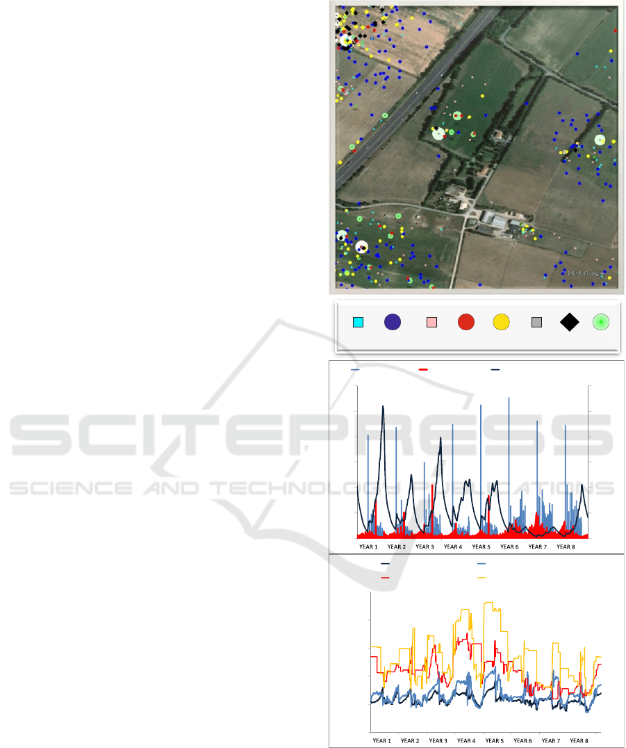
A common simulation output is presented on

Figure 2. Rodents distribute themselves through

time depending on the reproduction season and the

evolution of the field statuses. They usually

preferentially occupy perennial fields of meadow

or alfalfa as well as roadside verges or field borders

as described in the literature (e.g., Briner et al.,

2005, Topping et al., 2010). Population size (

Figure

2 middle) shows a seasonal fluctuation with births

occurring during the reproduction season. Mortality

peaks occur when ploughing happens in a crop

occupied by a colony of rodents. At a yearly scale,

population may undergo acute decline (e.g., year 7)

leading to either population collapse or restoring.

Mean dispersal (

Figure 2 bottom) remains steady

and fits with the observed vital domain of this

species (Quéré and Le Louarn, 2011), maximum

dispersal fluctuates at a value near the simulated

domain side with less dispersal for females which

remain more sedentary because of their childcare

activity.

2.3 Time Scale Mechanisms Involved

Three major categories of processes are bound to the

time scale used and vary accordingly to the time step

chosen for simulation. The first involves the duration

of each phase of the rodent life cycle (weaning,

maturity, gestation length, etc.); the second concerns

agents’ sensing:

Figure 2: standard simulation outputs of the studied use

case - common vole rodents in a fragmented agricultural

landscape. Top: snapshot of the population distribution

within the simulated domain; middle, population size and

birth/death rates; bottom: evolution of mean and

maximum dispersal within the period (simulation time

step: 3hours).

♂♂

immature mature

♀♀♀

immature mature pregnant suckli ng dispersing burrow

system

200

400

600

800

1000

1200

10%

20%

30%

40%

50%

60%

birth rate (%) death rate (%) Population size (right axis)

100

150

200

250

meters

meanFemaleDispersal meanMaleDispersal

maxFemaleDispersal maxMaleDispersal

Using Flexible Time Scale to Explore the Validity of Agent-based Models of Ecosystem Dynamics: Application to Simulation of a Wild

Rodent Population in a Changing Agricultural Landscape

299

Agents have a sensing area encompassing any

object or agent (substrate nature, relatives, burrow

systems) perceptible within one time step. It is

defined as a fixed circle with a parameterized radius

(e.g., Jia et al., 2018) corresponding to the vital

range of this type of animal (Quéré and Le Louarn,

2011). The sensing area moves with the agent and is

computed precisely from the continuous space

coordinates. The radius value is declared in m/day

and is adjusted to the time step (or tick) scale used

by converting it into m/tick or cell/tick depending on

the behaviour mechanism involved in rodent’s

activity.

The third category of process depending on

time scale is the common speed of the agent which

is also expressed in m/day and converted into

m/tick. For a given time step, the rodent speed is

fixed except in cases where either its current place

has exceeded the cell or burrow system carrying

capacity or if it arrived in a dangerous area (e.g.,

road, motorway…). In such cases the rodent flees

from its current place at a speed four times its

normal speed until it reaches a place that is not

overloaded.

2.4 Flexible Time-scale Implementation

To ensure the integrity of the multiple scales units

and conversions dealt with and secure model’s

verification, we have first suffixed most methods or

properties names with the units that characterize

them (e.g., meter, day, cell, tick, gramPerDay).

Time and space conversion is realized using an

extension of the standard java Gregorian calendar

which constitutes the time reference within the

model. This class manages both a time amount and

a time unit (e.g., 3+hours). We also plugged a

converter class providing all the necessary utilities

to operate the needed conversions between time

step units and universal units managed by the

calendar. This permits conversion of speeds and

sensing spheres depending of the time or space

units in the continuous space and within the grid

(e.g., meter per day into meter per tick or into grid

cells per tick).

2.5 Simulation Conditions and

Sensitivity Analysis Performed

The rodent population is initialized with 400

individuals and 50 burrow systems representing a

pioneer population density of 25 ind./ha.

Simulations are run using time steps ranging (i) from

5 min to 90 min each 5 min, (ii) from 90 min to 48

hours each 10 min and (iii) from 48 hours to 9 days

each 30 min. Two constraints are imposed to stop

simulations. The first correspond to a maximum of

three years simulation duration, giving a one-year

cycle to allow the model to escape from initial

conditions and two supplementary yearly cycles

with similar cyclic patterns. Simulations are stopped

at the beginning of the reproduction season where

rodents’ population is at its lowest. The second stop

condition is triggered when either a maximum

population of 6.000 individuals evolving within the

domain is reached, that is a signature of a pullulating

population, or when no female remains, hence

signing a collapsing population. Two indicators are

selected to study the effect of changing time step,

the first one is the duration of the simulation; either

max allowed time or population life before collapse.

The second is the size of the population at the end of

the simulation

3 RESULTS

Depending on the initial parameter values the

simulated population may persist a few days to

several centuries before collapsing. In the current

model the latter case is rare and the population often

collapses in the complex environment within which

it evolves. This is expressed in Figure 3 where the

time step values tested almost always result in the

early extinction of the population, except for small

tick values.

The range of values used in this sensitivity

analysis is intentionally larger than the supposed

realistic range of time step values; this makes it

possible to highlight the artefactual behaviours

related to the model function and the simplification

that it brings. Thus, the right of the graph shows an

increase in the lifetime of the population as the

time step increases with a phase transition at a time

step of 190 hours leading to a plateau. In those

extreme situations from 20 to 190 hour per time

step, the increase in the population life span is

related to the increase in rodent speed and

perception that allows them to reach their target

more and more quickly during a single cycle (as of

a time step equals to 63 hours, rodents acquire a

complete perception of the domain at each tick).

Detailed simulations observed there indicate a

boundary conditions effect that becomes

preponderant with a significant rodent density

observed abutting the limits of the domain.

SIMULTECH 2018 - 8th International Conference on Simulation and Modeling Methodologies, Technologies and Applications

300

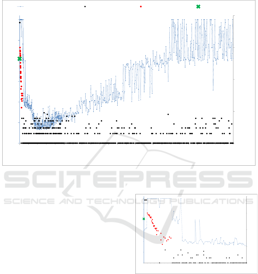
Figure 3: Selected output indicators of the time step sensitivity analysis. Dots: population size at the end of the simulation;

dotted line: duration of the simulation. Simulations are stopped when the rodent population collapses, when it exceeds 6.000

individuals (proliferation), or when the duration reaches 3 years.

The last plateau to the right of the figure starts at

the time step 190 hours when rodents acquire a

speed per tick allowing them to traverse the whole

domain modelled during a single time step. At this

stage, any target is instantly reached. However, this

functionality does not allow the population to persist

and in this value range no population is viable. The

observed outputs indicate high mortality peaks

during the winter season. These peaks are attributed

to the non-optimal positioning of rodents related to

their excessive displacements.

For much shorter time steps (Figure 4),

simulations indicate a range of tick values (in red)

that enables a sustainable population over the

medium term (i.e., beyond the period presented

here). Within this interval, the population remains at

a sufficient level to resist the hazards of its

environment. This range of values also reflects the

adequate frequency of agents’ deliberation/execution

process. It lies in this case between 25 minutes and 3

hours with optimal value at about 45 min

corresponding to an almost steady population (see

illustration on Figure 2).

Figure 4: Sensitivity analysis outputs for small values of

the time step: focus on the extreme left part of Figure 3;

same caption used.

It can be also noticed that within this interval, the

more the time step increases, the more the dynamics

of the population deteriorates with a smaller and

smaller size at the end of the simulation. This

phenomenon can be attributed to a less efficient

adaptation of the virtual population to its simulated

environment. It can be also interpreted as a bias

related to the method used for computing the

100

1 000

10 000

0.5

1.0

1.5

2.0

2.5

3.0

050100150200

Time step (hour)

Simulation length (year) Population size (log) Perennial population Initial population

100

1 000

10 000

0.5

1.0

1.5

2.0

2.5

3.0

024681012

Time step (hour)

Using Flexible Time Scale to Explore the Validity of Agent-based Models of Ecosystem Dynamics: Application to Simulation of a Wild

Rodent Population in a Changing Agricultural Landscape

301

rodents’ sensing area according to the time step,

which will be discussed in the next section.

For very small tick values (5 to 20 min), the

observed phenomenon is a rodent outbreak. Detailed

observation of each of these simulations (not

figured) suggests that, using these small tick values,

rodents’ moves remain very limited from one time

step to another. The burrow systems then constitute

foci where rodents maintain themselves in dense

groups that reproduce intensely. In addition, when

burrows are established in stable areas, resident

populations may be less subject to the hazards of the

environment than when they move further.

4 DISCUSSION

Performing a sensitivity analysis of the model on a

wide range of time scales provided two types of

insights. On the one hand it permitted to get better

understanding of the model function and limitations.

On the other hand it provided a mean to infer a

reasonable range of validity from the logic of the

modelled processes, such as here the frequency of

decision/action processes performed by rodents over

a period of time and leading to a perennial

population in a given environment. The valid range

of frequency here suggests that rodents in the wild

would perform a deliberation process from each 3

min to each 3 hours. To our knowledge, this value is

not accessible to experimentation or sampling.

However, it could constitute a clue to estimate the

order of magnitude of the cognitive activity that

these small animals realize in their environment.

Nevertheless, these results have to be considered

with caution and as only indicative since they come

from a single parameter sensitivity analysis, that is,

all other things being equal otherwise. It is almost

certain that the model is also sensitive to numerous

other aspects such as the spatial resolution or the

initial conditions imposed. Changing values for

these parameters would be susceptible to modify the

resulting optimal time scale that rose out of the

analysis. Multi-criteria sensitivity analysis (e.g.,

Saltelli et al., 2004) would therefore be necessary to

get more confident insight into the model’s

potential.

Simulations indicated large variation of the

selected indicator outputs; the population life time

and size. In an ideal scheme, the expected outcome

of such analysis would be that the simulated

population dynamics and indicator values would

remain unchanged whatever the time scale chosen.

Some contexts permits to reach such objective.

These occur when relationships between time

dependent parameters and time scale are linear. This

was here the case for life traits parameters such as

gestation, weaning duration, ageing.... Changing

time scale did not change the rodent agents’ life

cycle whatever the time step chosen. Kuo et al.

(2012) developed an epidemiological stochastic

agent-based model where probabilities could be

adjusted relative to time scale. In this case also, their

study led to almost reproducible results whatever the

time scale chosen. When however relationships

between time step and time-dependent parameters

are not linear, discrepancies appear and increasing

biases occur with increasing changes in time steps.

This is particularly the case here for time scaling

of agents’ perception area. Little literature was

found on formalization of agents' perception area.

Jia et al. (2018) used sensing circle radius as the

parameter defining the perception area of an agent.

This parameter was also used in this study to define

the agents’ sensing area and perform the conversion

from one time scale to the other. In a fixed time step

context, this approach is indeed the more logical and

straightforward. However, in a multi-time-scale

context, where sensing area must be scaled as a

function of time, it is not clear if this approach

comes out as a satisfactory solution. Geometry

calculations made before this study indicate that, in

the case of a straight line movement, the cumulated

area perceived by a rodent during several small time

steps is greater than that of a circle corresponding to

the area perceived on a larger time step equivalent to

the sum of the previous ones. At the same time, if

one considers that the rodent does not usually move

in a straight line but in an erratic or semi-erratic

trajectory such as in Lévy flight’s (Chechkin et al.,

2008), as it is the case during foraging, this travelled

area then decreases and converges toward the same

order of magnitude than the integrated circle.

In any case therefore, the area actually perceived

depends on the detail of the agent’s trajectory. It is

indeed logical that the perception area computed at

any timescale depends on the simulated trajectories

of rodents. Since these trajectories are moreover

themselves dependent on time and objects, changing

time scale produces biases in the model outcome

that may be difficult to reduce.

5 CONCLUSION

Exploitation of the model output at different time

scales proved valuable to better understand the

model potential, limitation and functioning. This

SIMULTECH 2018 - 8th International Conference on Simulation and Modeling Methodologies, Technologies and Applications

302

approach also provided a better insight on the

plausible range of activity of rodents in the wild

such as the frequency at which they should react to

their environment by mean of the perception/

deliberation scheme, within the limitation of such

simplified model.

This work also raises question on the best way to

formalize sensing. In this domain, comparative study

of different means to formalize time-dependent

perception, for example by using a surface, a radius,

or making agents’ sensing area a time-independent

parameter, would help improving modelling of

ecosystem-dependent agents.

ACKNOWLEDGEMENTS

The authors would like to thank S. Corso for his

contribution to the question of perception

formalization; J.P. Quéré, B. Gauffre, K. Berthier for

their expertise on the bio-ecology of the common

vole, P.A. Mboup for his implementation of the

space and time-scale converter, and S. Le Fur for

English verification. We gratefully acknowledge

support provided by CEA-MITIC (The African

Centre of Excellence in Mathematics, Computer

Science and ICT).

REFERENCES

Al Rowaei, A. A., Buss, A. H., and Lieberman, S., 2011.

The effects of time advance mechanism on simple agent

behaviors in combat simulations. Proc. Winter

Simulation Conference: 2431-2442.

Balci, O., 1998. Verification, Validation, and Accreditation.

Proc. Winter Simulation Conference: 41-48.

Briner, T., Nentwig, W. and Airoldi, J.P., 2005. Habitat

quality of wildﬂower strips for common voles (Microtus

arvalis) and its relevance for agriculture. Agriculture,

Ecosystems and Environment 105:173–179

Buss, A., Al Rowaei, A., 2010. A comparison of the

accuracy of discrete event and discrete time. Proc.

Winter Simulation Conference: 1468-1477.

Caillou, P., Gaudou, B., Grignard, A., Truong, C. Q. and

Taillandier, P., 2017. A Simple-to-use BDI architecture

for Agent-based Modeling and Simulation. Advances in

Social Simulation 2015:15-28.

Chechkin, A., Metzler, R., Klafter, J. Gonchar, V., 2008.

Introduction to the Theory of Lévy Flights. In R.

Klages, G. Radons, I.M. Sokolov (Eds), Anomalous

Transport: Foundations and Applications, Wiley-VCH,

Weinheim.

DeAngelis, D. L., Mooij, W. M., 2003. In praise of

mechanistically rich models. In: Canham, C. D., Cole, J.

J., Lauenroth, W. K. (Eds.), Models in Ecosystem

Science. Princeton University Press, Princeton, New

Jersey, pp. 63–82.

Ferber J., 1999. Multi-agent systems: an introduction to

distributed artificial intelligence, Addison-Wesley

Reading.

Ferber, J. and Müller, J. P., 1996. Influences and reaction: a

model of situated multi agent systems. Proc.

International Conference on Multi-Agent Systems

(ICMAS-96): 72-79.

Floudas, C. A., and Lin, X., 2004. Continuous-time versus

discrete-time approaches for scheduling of chemical

processes: a review. Computers & Chemical

Engineering, 28(11): 2109-2129.

Fu, Z., Hao, L., 2018. Agent-based modeling of China’s

rural-urban migration and social network structure.

Physica A: Statistical Mechanics and its Applications:

1061-1075.

Jia, J., Chen, J., Chang, G., Wen, Y., and Song, J., 2009.

Multi-objective optimization for coverage control in

wireless sensor network with adjustable sensing radius.

Computers & Mathematics with Applications, 57(11-

12), 1767-1775.

Kuo, C. T., Wang, D. W., and Hsu, T. S., 2012. A Simple

Efficient Technique to Adjust Time Step Size in a

Stochastic Discrete Time Agent-based Simulation. In

Proceedings of the 2nd International Conference on

Simulation and Modeling Methodologies, Technologies

and Applications - Volume 1: SIMULTECH: 42-48.

Le Fur, J., Mboup, P.A., and Sall, M., 2017. A Simulation

Model for Integrating Multidisciplinary Knowledge in

Natural Sciences. Heuristic and Application to Wild

Rodent Studies. Proc. 7th Internat. Conf. Simul. And

Model.Method., Technol.and Applic. (Simultech),

Madrid, july 2017: 340-347.

North, M. J., Howe, T. R., Collier, N. T., Vos, J. R., 2005.

The Repast Simphony Development Environment. In,

Proc. Agent 2005 Conference on Generative Social

Processes, Models, and Mechanisms:13-15.

Ponomarenko, A., and Sinyakov, A., 2018. Impact of

Banking Supervision Enhancement on Banking System

Structure: Conclusions Delivred by Agent-Based

Modelling. Bank of Russia Working Paper Series

wps19, Bank of Russia.

Quéré, J.P. and Le Louarn, H., 2011. Les rongeurs de

France: faunistique et biologie. Quae ed., Paris, ISBN:

978-2-7592-1033-6, 312p.

Railsback, S., Ayllón, D., Berger, U., Grimm, V., Lytinen,

S., Sheppard, C., and Thiele, J., 2017. Improving

execution speed of models implemented in NetLogo.

Journal of Artificial Societies and Social Simulation,

vol. 20, no. 3. doi:10.18564/jasss.3282

Saltelli, A., Tarantola, S., Campolongo, F., Ratto, M., 2004.

Sensitivity Analysis in Practice. Wiley, New York.

Sauser, B., Baldwin, C., Pourreza, S., Randall, W., and

Nowicki, D., 2018. Resilience of small-and medium-

sized enterprises as a correlation to community impact:

an agent-based modeling approach. Natural Hazards,

90(1): 79-99.

Singh, K., Ahn, C. W., Paik, E., Bae, J. W., and Lee, C. H.,

2018. A Micro-Level Data-Calibrated Agent-Based

Using Flexible Time Scale to Explore the Validity of Agent-based Models of Ecosystem Dynamics: Application to Simulation of a Wild

Rodent Population in a Changing Agricultural Landscape

303

Model: The Synergy between Microsimulation and

Agent-Based Modeling. Artificial life: 128-148.

Squazzoni, F., 2010. The impact of agent-based models in

the social sciences after 15 years of incursions. History

of economic ideas: 197-233.

Stanilov, K., 2012. Space in agent-based models. In Agent-

based models of geographical systems: 253-269).

Springer, Dordrecht.

Topping C. J., Høye T. T. and Olesen C. R., 2010. Opening

the black box – development, testing and documentation

of a mechanistically rich agent-based model. Ecological

Modelling 221 (2) 245-255.

Watts, J., 2016. Scale Dependency in Agent-Based

Modeling: How Many Time Steps? How Many

Simulations? How Many Agents?. Uncertainty and

Sensitivity Analysis in Archaeological Computational

Modeling, Springer, Cham.: 91-111.

White, A. A., 2016. The sensitivity of demographic

characteristics to the strength of the population

stabilizing mechanism in a model hunter-gatherer

system. In Uncertainty and Sensitivity Analysis in

Archaeological Computational Modeling, Springer,

Cham.: 113-130.

Whitley, T. G., 2016. Archaeological simulation and the

testing paradigm. In Uncertainty and Sensitivity

Analysis in Archaeological Computational Modeling

Springer, Cham.: 131-156.

SIMULTECH 2018 - 8th International Conference on Simulation and Modeling Methodologies, Technologies and Applications

304