
Compliance Error Compensation based on Reduced Model for
Industrial Robots
Shamil Mamedov, Dmitry Popov, Stanislav Mikhel and Alexandr Klimchik
Institute of Robotics, Innopolis University, Universitetskaya Str. 1, Innopolis, Russia
Keywords: Elastostatics, Virtual Joint Method, Industrial Manipulators, Machining, Deflection Compensation.
Abstract: In the near future industrial manipulators can completely replace bulky and expensive CNC machines. The
only issue that stands in a way of this transition is low stiffness of industrial robots. However, a lot of
research is going on in this area with the focus on developing an accurate stiffness model of the robot and
embedding it into the control scheme. The majority of the stiffness models include stiffness of the links as
well as joints even though typically complete link parameters are not provided by the robot manufacturers.
Therefore, it is of great importance to understand how accurately a reduced stiffness model which takes into
account only joint stiffness can replicate the results of the full model. In this paper, we focus on analyzing
the quantitative difference between these two models using Virtual Joint Modeling method and its effect on
trajectory tracking. The systematic analysis demonstrates that reduced stiffness model can quite accurately
replicate the full one and with reduced model, up to 95 percent of the end-effector deflection can be
compensated so that the average deflection error after compensation is about 0.8 tor a typical heavy
industrial robot under the loading.
1 INTRODUCTION
Nowadays there is a tendency to replace computer
numerical control (CNC) machines with industrial
robots as the latter are cheaper and occupy less
space. However, due to open-loop chain structure,
the stiffness of industrial robots is lower than of
CNC machines. Both theoretical and experimental
studies show that this ratio can be more than 50
times (Pan et al., 2006). Deformations due to low
stiffness lead to poor machining quality and
decreased processing efficiency (Zhang et al., 2005).
In order to bring accuracy of manipulators close to
the accuracy of CNC machines, researchers tend to
model robot elasticity and compensate related
compliance errors. For the stiffness modeling three
main approaches are distinguished in literature: the
finite elements analysis (FEA) (Taghaeipour et al.,
2010), the matrix structural analysis (MSA) (Martin,
1966) and the virtual joint method (VJM) (Klimchik
et al., 2017; Pashkevich et al., 2009; Pashkevich et
al., 2011) each of them have their own advantages
and disadvantages. Compliance error compensation
is a complicated problem since compensation in the
Cartesian space is achieved evidentially by the
motors located at the joints and naturally, the
following question arises: how accurately total
compliance – compliance of the links and joints –
can be lumped in the joints and dealt with?
To address this issue, the remainder of the paper
is organized as follows. Section 2 defines theoretical
models used in this paper. Section 3 describes a
model of the robot. In Section 4 results of
simulations are given. Section 5 provides discussion
and Section 6 summarizes main contributions of the
paper.
1.1 Related Work
Stiffness modeling of robotic manipulators was
initiated in the 1980s by a pioneering work of
Salisbury on active stiffness control (Salisbury,
1980). First models were taking into account only
joint elasticities and the stiffness parameters were
estimated in a straightforward way (Pigoski et al.,
1998). Recent developments in this field make it
possible to model both joint and link flexibility
(Klimchik et al., 2014), resulting in three main
approaches mentioned in the previous section. The
basic idea behind the FEA is to decompose the
physical model of a mechanism into a number of
small elements and to introduce compliant relations
between adjacent nodes by corresponding stiffness
180
Mamedov, S., Popov, D., Mikhel, S. and Klimchik, A.
Compliance Error Compensation based on Reduced Model for Industrial Robots.
DOI: 10.5220/0006905701800191
In Proceedings of the 15th International Conference on Informatics in Control, Automation and Robotics (ICINCO 2018) - Volume 2, pages 180-191
ISBN: 978-989-758-321-6
Copyright © 2018 by SCITEPRESS – Science and Technology Publications, Lda. All rights reserved

matrices (Corradini et al., 2003). Although this
method is highly accurate, as a number of finite
elements increase limitations of computer memory
and high dimension matrix inversion becomes
pressing. The MSA uses the main ideas of the FEA
but handles large complaint elements which lead to
reduced computational efforts (Martin, 1966).
Nevertheless, this approach is hardly applicable for
the manipulator in the loaded condition (Klimchik et
al., 2012). The last method and the one used in this
work is the VJM. It is based on the expansion of the
traditional rigid-body model of the robotic
manipulator with virtual joints corresponding to the
compliances of the links and joints (Pashkevich et
al., 2009). The use of VJM in justified by its
computational efficiency and acceptable accuracy.
The VJM model requires the parameters of
virtual springs in order to compensate the end-
effector deflections which are a priori unknown. As
in case of the model there are several ways to solve
this problem. First one is to approximate links by
symmetrical beams and use well-known equations to
compute the stiffness. But this method is rather an
oversimplification of the problem at hand and will
not result in accurate deflection compensation.
Another approach is to use CAD model of the
manipulator (Pashkevich et al., 2011). However, this
method is limited due to non-homogeneity and
variations in the material properties. Moreover,
CAD models are not provided by the robot
manufacturers. The last and seemingly the most
reliable approach is to exploit model calibration
techniques using the data from the real experiments
(Alici and Shirinzadeh, 2005; Nubiola and Bonev,
2013). Since the main goal is to compensate the
deflections as much as possible the parameters of the
virtual springs should be close to the real ones as
much as possible, consequently, the method based
on the real experiments is used in this work.
Once the full geometric model of the
manipulator including stiffness model is known, one
can try to compensate the deflections due to link and
joint flexibility. There are two main approaches –
online and offline compensations. First one involves
modification of the control algorithm by tweaking
the manipulator inverse/direct kinematics embedded
in robot software (Guillo and Dubourg, 2016; Zhang
et al., 2005). The second one is to modify the
reference trajectory. Usually, robot manufacturers do
not provide access to inner control algorithms
therefore in most of the cases user is left with the
second option. Therefore, it is not surprising that
off-line trajectory modifications are mainly applied
in the engineering practice (Belchior et al., 2013;
Olabi et al., 2012; Ozaki et al., 1991; Popov et al.,
2017). Among the most popular implementations of
off-line compensation is so-called “mirror
technique” (Chen et al., 2013), where the reference
and non-compensated trajectories are symmetrical
with respect to the desired one.
1.2 Problem Statement
Estimating all the stiffness parameters including
both link and joint stiffness’s from experiments is a
very challenging task as it requires identification of
more than 200 parameters for 6 DoF industrial robot.
But is it necessary to estimate them all considering
possibility to obtain them from the real experimental
data (Klimchik et al., 2015). If the overall stiffness
of the joints and links are lumped in the joints only
how precise the compensation of the end-effector
position due to machining or other industrial
processes will be? It is the main question of interest
of this work which will be systematically analyzed
in the following sections.
2 THEORETICAL
BACKGROUND
2.1 Virtual Joint Method
VJM is one of the approaches to develop detailed
and complete geometric model of the manipulator
which provides more accurate estimates of the end-
effector position and orientation. To do so, the
original model is complemented by virtual joints
which describe the elastic deformations of the links.
Moreover, virtual springs are included in the
actuated joints, in order to take into account the
stiffness of the transmission and control loop. As a
result, a so-called extended geometric model of the
robot is obtained (Eq. (1))
=
,
(1)
where is the vector of actuator coordinates and
is the vector of virtual joint coordinates. The values
of coordinates are completely defined by the robot
controller, while the values of virtual joint
coordinates depend on the external loading
applied to the robot end-effector.
Although the mathematical derivation of the
expression for deflection and Cartesian stiffness
matrix has been shown in several papers, for
completeness of the VJM it is provided here as well.
Variations in the virtual joint variables generate
Compliance Error Compensation based on Reduced Model for Industrial Robots
181

the reaction forces/torques in the corresponding
links that are evaluated by the generalized Hooke's
law for the manipulator in virtual joints space
=
(2)
where
is the vector of torques generated in virtual
joints,
=
,
,…,
is overall virtual
joint stiffness matrix and
is the spring stiffness
matrix of the corresponding link/joint.
By applying the principle of virtual work and
assuming that displacements in the virtual joints Δ
are small, we obtain the virtual work done by the
external wrench
=
Δ
(3)
where
=
,
⁄
is the Jacobian matrix
with respect to .
On the other hand, for the internal forces
, the
virtual work is equal to
=−
Δ
(4)
As in the static equilibrium the total virtual work is
equal to zero for any virtual displacement, the
equilibrium conditions can be derived as
=
(5)
Combining (2), (5) and linearizing (1) around the
equilibrium point, the equation for the end-effector
deflection can be obtained
∆=
(6)
From Eq. (6) an expression for Cartesian stiffness
matrix can be extracted
=
(7)
The relationship between the Cartesian and joins
spaces proposed in (Zargarbashi et al., 2012) is
called the conservative congruence transformation
(CCT).
2.2 Identification
To estimate the compliances of virtual springs it is
more convenient to rewrite Eq. (6) in a form
∆=
∑
,
,
,
(8)
where is number of measurements, the matrices
denote the link/joint compliances to be
identified, and
denote sub-Jacobians -
=
[
,
,
,
…]. Further, to represent the model in a
form standard for identification – as a linear function
with respect to parameters to be identified, the Eq.
(8) is rewritten as
∆=
,
(9)
where
=[
,
,
,…,
,
,
] is so-called
observation matrix and =
,
,
,
,…,
,
.
The optimization problem for compliance matrix
identification is posed as
‖
Δ
−
,
‖
→
(10)
where the index defines the manipulator
configuration number.
3 MODEL DESCRIPTION
As it was mentioned before the virtual joint method
is the most appropriate method for the manipulator
stiffness modeling (Klimchik et al., 2014). In the
frame of this approach, several alternative
techniques have been proposed. They differ in a
number of parameters and dimensions of virtual
springs describing the link/joint elastostatic
properties. To be more specific, let us consider
KUKA KR270 robotic manipulator
(Fig. 1)
performing any machining operation. It consists of a
fixed base, a serial chain of flexible links, a number
of flexible actuated joints, the end-effector which is
in contact with a workpiece undergoing machining
and an external wrench applied to it due to the
technological process. To build full stiffness model
of the robot, VJM proposes to model the stiffness of
each link with 6 DoF spring, three of which
correspond to translation and three to the rotation
and the joint with 1 DoF spring positioned along the
axis of rotation of the joint (Fig. 2d). In this case
stiffness matrix of the manipulator
has the
dimension 3636. To use this model, more than
250 parameters should be known (Klimchik et al.,
2013). In an ideal scenario, these parameters can be
obtained from CAD model of the given robot,
however in reality it is hardly possible. Thus, a lot of
effort was put in order to construct simpler models
which can provide results close enough to full
model.
ICINCO 2018 - 15th International Conference on Informatics in Control, Automation and Robotics
182
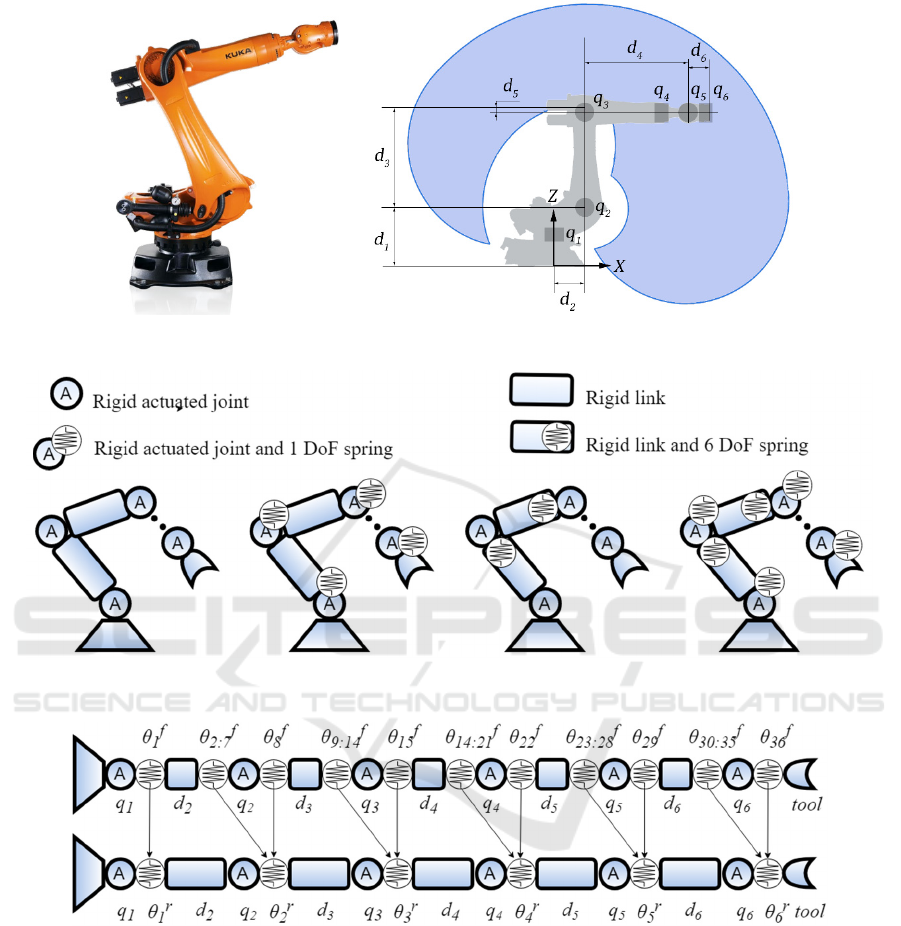
Figure 1: KUKA KR270 and its kinematic scheme with the workspace.
a) Rigid joints and links b) Rigid links and flexible
joints
c) Flexible links and rigid
joints
d) Flexible links and
joints
e) Full and reduced models
Figure 2: Possible VJM models for four different cases.
For developing reduced stiffness model there are
three main approaches. The first one is used when
the stiffness of the joints is much higher than the
stiffness of links, therefore the joints can be
considered as rigid (Fig. 2c). For this reduced model
the stiffness matrix
is of dimension 3636.
The second approach is used when the opposite is
true i.e. the stiffness of the link is much higher than
the stiffness of the joints, thus the links are taken as
rigid (Fig. 2b). In this case the stiffness matrix
is
of dimension 66 and diagonal. The last approach
is used when the stiffness of the links is higher than
of the joints but not negligible. Here, part of a link
stiffness is incorporated into the stiffness of the
corresponding joint. As in case of
the size of the
stiffness matrix
is 66 and it is diagonal.
The first approach is very rarely used in
industrial framework because links of industrial
robots are stiff, in addition to that it requires CAD
model. Regarding the second approach, links are
Compliance Error Compensation based on Reduced Model for Industrial Robots
183
usually not rigid enough to neglect them. This model
is used in this work to understand the contribution of
each elastic component to overall stiffness matrix.
The main analysis was performed on full model and
reduced model. From now on the reduced model
implies the one obtained by the third approach. In
the cases when we refer to other reduced models it
will be mentioned explicitly.
Table 1: Geometric parameters of the links.
Parameter
Length,
m
Outer
diameter,
m
Inner
diameter,
m
0.675 0.35 0.30
0.35 0.35 0.30
1.15 0.35 0.30
1.2 0.25 0.20
0.041 0.25 0.20
0.24 0.25 0.20
By using the geometric and virtual springs
parameters (Tables 1 and 2) of the KUKA KR270
,
its extended geometric model can be developed for
full (Eq. (11)) and reduced (Eq. (12)) elastostatic
models
=
:
:
:
−
:
:
(11)
=
−
(12)
where
is a homogeneous transformation matrix
with translation in u direction,
is a homogeneous
transformation matrix with rotation about u axis,
is a homogeneous transformation matrix with
all 6 translation and rotation components. Both
models are also presented in Fig. 2e.
Table 2: Joint stiffness values and upper and lower limits.
Joint № Compliance um/N
Lower
limit, deg.
Upper
limit, deg.
1 0.4 -179 179
2 0.28 -50 90
3 0.28 -155 120
4 2.5 -350 350
5 2.8 -122 122
6 2 -350 350
Table 3: Identified joints compliances of the manipulator.
Joint №
1 2 3 4 5 6
,
/
0.56 0.30 0.43 2.8 3.2 2.1
3.1 Stiffness Estimation
The process of stiffness identification consists of
two steps. First one is displacement modeling. Here
it is assumed that both joints and links are elastic
and influence the end-effector position. In order to
find the value of the displacement, system Jacobian
for the given configuration is required (Eq. (6)). It
can be obtained from the solution of the forward
kinematic problem. If the Jacobian and virtual joint
stiffness matrices are known, then the vector of
displacement can be calculated using Eq. (8).
The second step is robot calibration. During this
step it is assumed that joints are elastic while links
are rigid, i.e. try to find an equivalent manipulator
with elastic joints that have the same displacement
parameters as the initial robot. Thus, only the
actuator stiffness values have to be identified.
Identification process requires the measurements
of the end-effector in different configurations and
under the various force orientation. Mathematical
model allows to sequentially check all possible
states in robot workspace, but this is not necessary.
In experiments, random joint angles were generated
and force with arbitrary orientation and a constant
value of 10
N was applied to the end-effector. The
process terminated when the relative error of one
iteration was less than a predefined threshold (about
0.01%). Obtained results are represented in Table 3.
Cartesian compliance matrix
which is the
inverse of the cartesian stiffness matrix,
sets the
relationship between the generalized displacement of
the end-effector and external wrench applied to it
(Eq. (6-7)). The problem with
is that it has
elements with different physical units. It causes
difficulties in analyzing compliance of the robot.
However, it was shown in (Zargarbashi et al., 2012)
ICINCO 2018 - 15th International Conference on Informatics in Control, Automation and Robotics
184

that in machining operations the rotational
displacement of the tool can be negligible compared
to its translational displacement. Thus, the analysis
of generalized end-effector displacement can be
reduced to the analysis of its translational
displacement, so that Eq. (6) and Eq. (7) combined
become:
∆
0
=
0
(13)
where ∆=
[
∆
∆
∆
]
and =
[
]
. Compliance matrix
can be
divided into four submatrices (Guo et al., 2015):
=
,
,
,
,
(14)
where
,
is the translational compliance
submatrix,
,
is the rotational compliance
submatrix, and
,
is the coupling compliance
submatrix.
By substituting Eq. (14) into Eq. (13) a direct
relationship between ∆ and can be obtained
∆=
,
(15)
Eq. (15) is used further in this paper in order to build
deflection maps.
3.2 Deflection Maps
When the joint stiffness values are known,
distribution of deflection in the robot workspace
(deflection map) can be built. Such maps could be
calculated, for example, along the end-effector
trajectory or for some workspace plane. Both
representations are considered in this work.
There are several problems that can be
encountered during these computations. One of them
is a robot configuration as it is obvious that parts of
the workspace can be reached using several
configurations, while other parts only by one
combination of joint angles. Each configuration is
characterized by its own stiffness, so the question is
which one should be used for computation? This
problem does not have much sense for the given
robot in case of operation in XOY plane because
each point can be reached without changing
manipulator configuration. But in the orthogonal
plane (XOZ) in order to obtain highest or lowest
points of workspace configuration must be changed.
For the manipulator used for simulations and
represented in Fig. 2, there are two main
configurations: “elbow up” – when the angle
is
negative and “elbow down” – when
is positive.
In the horizontal plane, for the sake of simplicity,
only one of them, “elbow up” is considered as it is
more common. In case of the vertical plane, two
deflections for different workspaces should be
combined. It is assumed that manipulator will
operate in optimal mode hence minimal deflection
should be chosen in the intersection of two regions.
The second problem is the value and direction of
the applied force which could provide the worst
result, i.e. maximum deflection. This problem can be
solved by exploiting the singular value
decomposition (SVD) method (Leon, 1980) applied
to the translational compliance submatrix (Eq. (15)).
,
=
(16)
where the diagonal elements of are nonnegative
singular values in decreasing order, the columns of
are left singular vectors and columns of are
right singular vectors.
The first element of the matrix is an absolute
value of the maximal deflection obtained under the
influence of a unit force (1 N). Direction of this
deflection is corresponding left singular vector i.e.
first column of matrix . The similar approach was
used in (Guo et al., 2015).
4 RESULTS
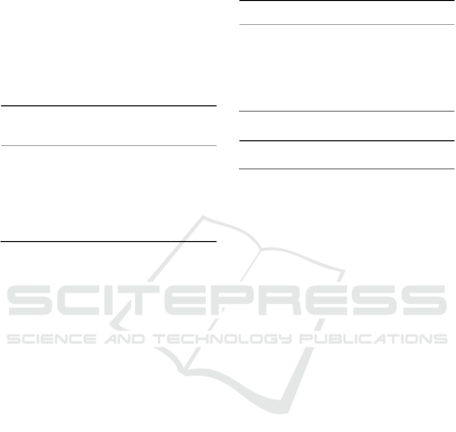
4.1 Deflection Maps
Deflection maps for the manipulator with the full
elastostatic model are shown in Fig. 4. Upper image
corresponds to the vertical plane at the 0.5 m level.
The map demonstrates radial symmetry, deflection
grows with distance and increases from the center to
the edges due to increase in the lever length. As in
case of the horizontal plane, the deflection increases
proportionally to the distance from the origin of the
base link due to the same reason. Here no symmetry
can be spotted as the second and third joint limits are
not symmetrical with respect to the Z axis.
Maximum deflection that manipulator undergoes
under the unit force applied in the direction leading
to maximum deflection for both vertical and
horizontal planes is 4 . The sudden change of the
deflection along X-axis corresponds to the change
from the configuration “elbow up” to “elbow down”.
Deflection maps of the manipulator with the reduced
elastostatic model – the model which takes into
account only estimated joint elasticities, obtained
from the calibration process (Table 3) are shown in
Figure 4.
Compliance Error Compensation based on Reduced Model for Industrial Robots
185
a) Horizontal plane
b) Vertical plane
Figure 3: Deflection maps for the manipulator with full
elastostatic model.
a) Horizontal plane
b) Vertical plane
Figure 4: Deflection maps for the manipulator with
reduced elastostatic model.
a) Vertical plane b) Horizontal plane
Figure 5: Error histograms of the full and the reduced models.
ICINCO 2018 - 15th International Conference on Informatics in Control, Automation and Robotics
186
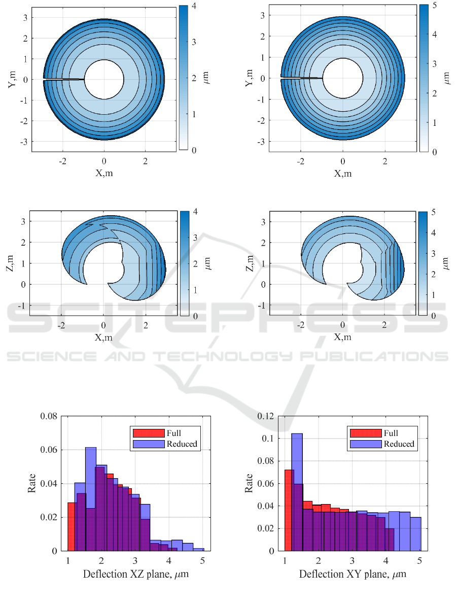
a) Horizontal plane
b) Vertical plane
Figure 6: The difference in the deflection maps of the
manipulator with full and reduced model.
It is rather obvious that reduced model deflection
map is different from the full as the number of
elastic elements representing the manipulator is
decreased. However, the difference is not significant
because experiment based compliance identification
of the joint parameters incorporates some of the link
parameters. For this reason, the reduced model can
provide results accurate enough to be used in the
compensation process. To understand the degree of
accuracy the difference between full and reduced
model deflection maps is provided in the Fig. 6.
Fig. 6 shows that the maximum difference is 0.8
(84%) and concentrated on the particular region.
It is explained by the chosen approach where we
apply unit force along the direction of maximum
deflection extracted from the full model as it better
describes elasticity of the manipulator. The simple
conclusion that can be drawn from the difference
map is that the reduced model is very good in
recovering the performance of the full model for the
setup considered in this paper while requiring many
fewer parameters (Fig. 5 demonstrates that error
distributions are almost the same).
4.2 Deflection Compensation
In order to find an error of obtained model, we can
compare trajectories of the end-effector with and
without compensation for some technological
process. Assuming that the manipulator has to
move along the trajectory, shown in Fig. 7a, 8a
under the influence of the force =
[440,−1370,−635,0,0,0], cutting forces caused
by machining process (Klimchik et al., 2017). This
force makes the trajectory of the end-effector
different from the desired one. Depending on the
value and the orientation of the applied force, the
difference between trajectories can not only be
shifted but also has a different shape.
In order to compensate for the difference, the
deflection at each point should be found, using
reduced stiffness model of the manipulator. At this
point, widely used mirroring technique can be
utilized for compensation. New compensated
trajectory is used as an input of the manipulator
control system. The error between desired and
obtained trajectories for the robot without
compensation in every direction is shown in the Fig.
9b, 10b while the same figure but for the robot with
compensation is demonstrated in the Fig. 7c, 8c.
Mean and maximum errors for both cases are
presented in Table 4 and 5.
Table 4: Max and mean error for circle with 0.01m radius.
Direction
Uncompensated Compensated
Max
error,
mm
Mean
error,
mm
Max
error,
mm
Mean
error,
mm
X
0.779 0.776 0.114 0.113
Y
1.841 1.825 0.169 0.160
Z
0.639 0.628 0.019 0.017
Table 5: Max and mean error for circle with 0.5m radius.
Direction
Uncompensated Compensated
Max
error,
mm
Mean
error,
mm
Max
error,
mm
Mean
error,
mm
X
1.072 0.753 0.185 0.111
Y
2.838 1.968 0.622 0.314
Z
1.261 0.701 0.079 0.045
Compliance Error Compensation based on Reduced Model for Industrial Robots
187
a) Trajectories in the Cartesian space Green
dotted circle is uncalibrated trajectory, the
blue dash-dot circle is desired trajectory,
the red solid circle is a trajectory after
calibration process
b) Position error for the
uncompensated case. The red solid
line is an error in the X direction,
Green dotted line is an error in the
Y direction, Blue dash-dot line is
an error in the Z direction, the
Dashed line is error norm
c) Position error for the
compensated case. The red solid line
is an error in the X direction, Green
dotted line is an error in the Y
direction, Blue dash-dot line is an
error in the Z direction, the Dashed
line is error norm
Figure 7: Tool trajectories a circle with 0.5m radius.
a) Trajectories in Cartesian space Green
dotted circle is uncalibrated trajectory,
Blue dash-dot circle is desired trajectory,
the Red solid circle is a trajectory after
calibration process
b) Position error for the
uncompensated case. The red solid
line is an error in the X direction,
Green dotted line is an error in the Y
direction, Blue dash-dot line is an
error in the Z direction, the Dashed
line is error norm
c) Position error for the compensated
case. The red solid line is an error in
the X direction, Green dotted line is
an error in the Y direction, Blue dash-
dot line is an error in the Z direction,
the Dashed line is error norm
Figure 8: Tool trajectories for a circle with 0.01m radius.
For the small circle trajectory with 0.01m radius,
the maximum error is decreased by 85% in X, 91%
in Y and 97% in Z directions while for the large
circle maximum error is decreased by 83% in X,
78% in Y and 94% in Z directions. At the same time
mean error in case of the small circle was reduced
by 85%, 91% and 97% in X, Y and Z directions
correspondingly, while in case of the large circle
mean error was reduced by 85% in X, 84% in Y and
94% in Z directions. To be more concise, the
maximum and the mean norms of the error for large
circle were decreased by 80% and 84% respectively
while for small circle both by 90%. The numbers
demonstrate excellent quality of the compensation
even though it is based on the reduced model.
5 DISCUSSION
So far, the analysis was conducted for the
manipulator having geometrical properties of KUKA
KR270. Due to unknown internal structure of its
links, to develop full elastostatic model, we roughly
approximated all the links with hollow cylinders
with a wall thickness of 5cm. Thus, the results hold
true for this particular case and are not applicable to
ICINCO 2018 - 15th International Conference on Informatics in Control, Automation and Robotics
188
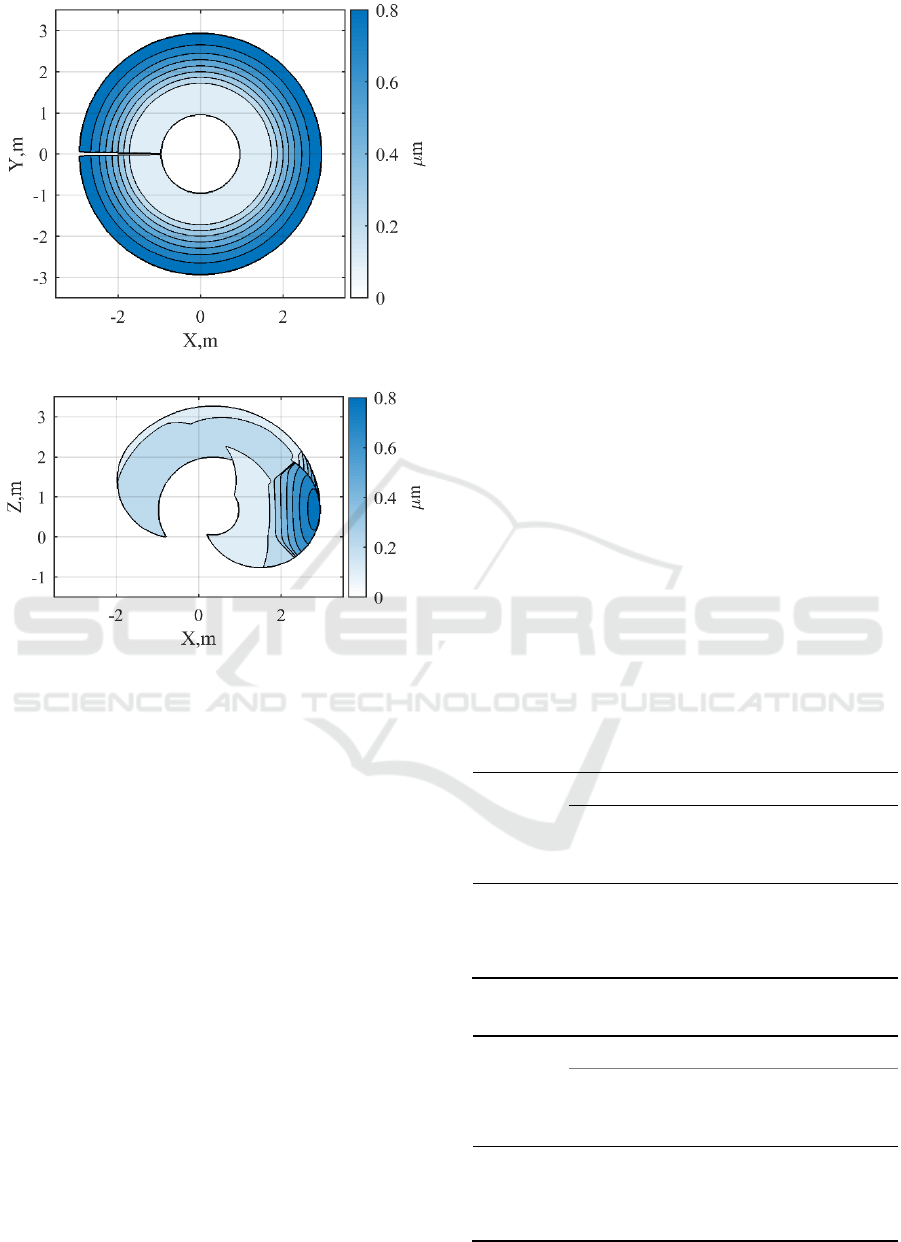
the generic manipulator. To generalize obtained
results, first, we define more practical workspace –
restricted workspace (Fig. 9), which has the same
contour as full one but is smaller as to avoid
singularities. Then, we vary the thickness of the
walls from one to ten centimeters, to understand how
it affects the quality of compensation in full and
restricted workspaces.
Figure 9: Full and restricted robot workspaces in XZ.
As the thickness of the walls decreases the
quality of compensation decreases as well. The
efficiency of the compensation for both workspaces
is especially sensitive to wall thickness in the range
from one to four centimeters (Fig. 10).
Figure 10: Compensation effectiveness for reduced model
depending on link thickness.
To explain this, we can carry out a simple
experiment which makes use of the first two reduced
models described in Section 3. The experiment is the
following, for the whole workspace compute
deflections by using full model, a reduced model
which assumes that links are rigid and reduced
model which assumes that joints are rigid. Then find
the mean value of the deflection for all three cases,
repeat the procedure for all the given values of wall
thickness. The ration between the mean values of a
reduced model and the full model will show the
contribution of the links or joints to overall
deflection (Fig. 11). As reduced models complement
each other to the full model, only one of them is
plotted and allows to understand the whole picture.
Figure 11: Contribution of the compliance of the links to
the overall deflection of the full elastostatic model.
When walls are thin, due to low stiffness they
have a great deal of contribution to overall
deflection. Although the reduced model used
throughout this work accounts for some compliance
of the links, it is not enough to provide good quality
of compensation.
Figure 12: Uncompensated deflection in the vertical plane.
Regarding the Fig. 10, the minimum deflection
of the overall workspace is more than of restricted
one, this rather unintuitive results can be explained
by Fig.12 which shows that the compensation in the
regions neglected in restricted workspace was very
Compensation, %
Compliance Error Compensation based on Reduced Model for Industrial Robots
189

good. Nevertheless, the mean value of compensation
is almost the same for both workspaces.
There are several remarks to be made. First, for
simplicity, we assume that the manipulator does not
have gravity compensator. Its presence slightly
complicates the analysis by making the stiffness of
the second joint a nonlinear function of angle
(Klimchik et al., 2013). Second, the metrics used in
this work are maximum and mean values of
deflection when we analyze workspace, and
maximum and mean values of errors in all X, Y and
Z direction when we consider the trajectory of the
end effector. The usage of other metrics can provide
slightly different results. Third, the orientation error
is neglected as the level of precision that is discussed
in this paper is used in the field of machining and it
was shown that for machining operations the
rotational displacement of the tool is negligible
(Zargarbashi et al., 2012). The last, while
performing deflection analysis for overall workspace
we did not assume any specific machining operation
for the sake of generality and used singular value
decomposition to define the direction of maximum
deflection for the full model and apply unit force
along this direction for both full and reduced model
in estimating deflection. However, for a specific
machining operation, the analysis can be
particularized by defining the force on the end-
effector due to machining.
In our simulation we use a large number of
configurations and end-effector loads in the
identification process, that is hardly implementable
in real life scenario. To reduce the number of
experiments and preserve resulting accuracy, the
design of experiment theory could be used
(Klimchik et al., 2015; Klimchik et al., 2012; Wu et
al., 2015).
6 CONCLUSIONS
In the majority of the studies focused on deflection
compensation of the industrial manipulators, authors
assume the links to be rigid. In this work, we focus
on understanding when this assumption holds true
and in which cases the compliance of the links
cannot be neglected. It was shown that when the
walls of the links modeled as hollow cylinders are
thin (up to 4cm) full elastostatic model should be
considered while when they are thick enough (4cm
and more) then depending on the actual thickness of
the walls reduced model can compensate more than
80% of overall deflections in general.
In our future work, we plan to consider the
efficiency of the proposed method in real industrial
applications. This will introduce additional
difficulties that affect output accuracy like the
presence of the measurement noise, greatly reduced
a number of experiments, dynamic components that
currently is not considered by our model.
ACKNOWLEDGEMENTS
This research has been supported by the grant of
Russian Science Foundation №17-19-01740.
REFERENCES
Alici, G., and Shirinzadeh, B., 2005. Enhanced stiffness
modeling, identification and characterization for robot
manipulators. IEEE Transactions on Robotics, 21,
554–564.
Belchior, J., Guillo, M., Courteille, E., Maurine, P.,
Leotoing, L., and Guines, D., 2013. Off-line
compensation of the tool path deviations on robotic
machining: Application to incremental sheet forming.
Robotics and Computer-Integrated Manufacturing, 29,
58–69.
Chen, Y., Gao, J., Deng, H., Zheng, D., Chen, X., and
Kelly, R., 2013. Spatial statistical analysis and
compensation of machining errors for complex
surfaces. Precision Engineering, 37, 203–212.
Corradini, C., Fauroux, J., Krut, S., and Company, O.,
2003. Evaluation of a 4-Degree of Freedom Parallel
Manipulator Stiffness. Proceedings of the 11th World
Congress in Mechanism and Machine Science, 5.
Guillo, M., and Dubourg, L., 2016. Impact and
improvement of tool deviation in friction stir welding:
Weld quality and real-time compensation on an
industrial robot. Robotics and Computer-Integrated
Manufacturing, 39, 22–31.
Guo, Y., Dong, H., and Ke, Y., 2015. Stiffness-oriented
posture optimization in robotic machining
applications. Robotics and Computer-Integrated
Manufacturing, 35, 69–76.
Klimchik, A., Ambiehl, A., Garnier, S., Furet, B., and
Pashkevich, A., 2017. Efficiency evaluation of robots
in machining applications using industrial
performance measure. Robotics and Computer-
Integrated Manufacturing, 48, 12–29.
Klimchik, A., Caro, S., and Pashkevich, A., 2015. Optimal
pose selection for calibration of planar anthropo-
morphic manipulators. Precision Engineering, 40,
214–229.
Klimchik, A., Chablat, D., and Pashkevich, A., 2014.
Stiffness modeling for perfect and non-perfect parallel
manipulators under internal and external loadings.
Mechanism and Machine Theory, 79, 1–28.
ICINCO 2018 - 15th International Conference on Informatics in Control, Automation and Robotics
190

Klimchik, A., Furet, B., Caro, S., and Pashkevich, A.,
2015. Identification of the manipulator stiffness model
parameters in industrial environment. Mechanism and
Machine Theory, 90, 1–22.
Klimchik, A., Pashkevich, A., and Chablat, D., 2013.
CAD-based approach for identification of elasto-static
parameters of robotic manipulators. Finite Elements in
Analysis and Design, 75, 19–30.
Klimchik, A., Wu, Y., Caro, S., Furet, B., and Pashkevich,
A., 2014. Accuracy improvement of robot-based
milling using an enhanced manipulator model. In
Mechanisms and Machine Science (Vol. 22, pp. 73–
81).
Klimchik, A., Wu, Y., Dumas, C., Caro, S., Furet, B., and
Pashkevich, A., 2013. Identification of geometrical
and elastostatic parameters of heavy industrial robots.
In Proceedings - IEEE International Conference on
Robotics and Automation (pp. 3707–3714).
Klimchik, A., Wu, Y., Pashkevich, A., Caro, S., and Furet,
B., 2012. Optimal Selection of Measurement
Configurations for Stiffness Model Calibration of
Anthropomorphic Manipulators. Applied Mechanics
and Materials, 162, 161–170.
Leon, S. J., 1980. Linear algebra with applications.
Macmillan New York.
Martin, H. C., 1966. Introduction to matrix methods of
structural analysis. McGraw-Hill.
Nubiola, A., and Bonev, I., 2013. Absolute calibration of
an ABB IRB 1600 robot using a laser tracker.
Robotics and Computer-Integrated Manufacturing, 29,
236–245.
Olabi, A., Damak, M., Bearee, R., Gibaru, O., and Leleu,
S., 2012. Improving the accuracy of industrial robots
by offline compensation of joints errors. In 2012 IEEE
International Conference on Industrial Technology,
ICIT 2012, Proceedings (pp. 492–497).
Ozaki, T., Suzuki, T., Furuhashi, T., Okuma, S., and
Uchikawa, Y., 1991. Trajectory control of robotic
manipulators using neural networks. IEEE
Transactions on Industrial Electronics, 38, 536–540.
Pan, Z., Zhang, H., Zhu, Z., and Wang, J., 2006. Chatter
analysis of robotic machining process. Journal of
Materials Processing Technology, 173, 301–309.
Pashkevich, A., Chablat, D., and Wenger, P., 2009.
Stiffness analysis of overconstrained parallel
manipulators. Mechanism and Machine Theory, 44,
966–982.
Pashkevich, A., Klimchik, A., and Chablat, D., 2011.
Enhanced stiffness modeling of manipulators with
passive joints. Mechanism and Machine Theory, 46
,
662–679.
Pigoski, T., Griffis, M., and Duffy, J., 1998. Stiffness
Mappings Employing Different Frames of Reference.
Mechanism and Machine Theory, 33, 825–838.
Popov, D., Klimchik, A., and Afanasyev, I., 2017. Design
and Stiffness Analysis of 12 DoF Poppy-inspired
Humanoid. In Proceedings of the 14th International
Conference on Informatics in Control, Automation and
Robotics (pp. 66–78).
Salisbury, J., 1980. Active stiffness control of a
manipulator in cartesian coordinates. Proc. IEEE
Conf. on Decision and Control (CDC), 19, 95–100.
Taghaeipour, A., Angeles, J., and Lessard, L., 2010.
Online computation of the stiffness matrix in robotic
structures using finite element analysis. Department of
Mechanical Engineering and Centre for Intelligent
Machines, McGill University, Montreal.
Wu, Y., Klimchik, A., Caro, S., Furet, B., and Pashkevich,
A., 2015. Geometric calibration of industrial robots
using enhanced partial pose measurements and design
of experiments. Robotics and Computer-Integrated
Manufacturing, 35, 151–168.
Zargarbashi, S. H. H., Khan, W., and Angeles, J., 2012.
Posture optimization in robot-assisted machining
operations. Mechanism and Machine Theory, 51, 74–
86.
Zhang, H., Wang, J., Zhang, G., Gan, Z., Pan, Z., Cui, H.,
and Zhu, Z., 2005. Machining with flexible
manipulator: toward improving robotic machining
performance. In Advanced Intelligent Mechatronics.
Proceedings, 2005 IEEE/ASME International
Conference on (pp. 1127–1132).
Compliance Error Compensation based on Reduced Model for Industrial Robots
191
