Model Predictive Path Integral Control for Car Driving with Dynamic

Cost Map

Alexander Buyval, Aidar Gabdullin and Alexander Klimchik

Robotics Institute, Innopolis University, 1 University Street, Innopolis, Russian Federation

Keywords:

Stochastic Control, Path Integral Control, Model Predictive Control, Dynamic Cost Map.

Abstract:

Path planning in a complex dynamic environment is one of the key subsystems in an autonomous vehicle. This

paper presents an extension of Model Predictive Path Integral (MPPI) control method which is able to take

moving objects into account while path planning and driving. To obtain real-time performance, cost map up-

date with respect to dynamic objects both as basic MPPI is implemented as a set of concurrent processes using

CUDA technology. The algorithm’s performance is demonstrated on a model of a stock car in a simulation

environment.

1 INTRODUCTION

Control systems of autonomous vehicles have signiﬁ-

cantly evolved in last decades. Nowadays millions of

kilometers were traversed by the selves-driving cars

developed by different research groups and technolo-

gical companies. However, most of the time autono-

mous cars are working under conditions that are far

from being critical. But in real conditions, it is hard

to avoid critical regimes due to several reasons: (I)

step-like change in friction coefﬁcient (II) unexpected

change in trajectories of other vehicles on the road.

At the same time, control of the car in critical and

close-to-critical conditions still is a challenging task.

Main problems arising here are (I) strict time con-

straints applied to decision making (II) uncertainties

and noise in the object of control and surroundings

(III) dynamic objects in the environment moving with

trajectories hard to predict.

A number of modern approaches to the control of

unmanned vehicles in particular and robotic systems

in general use the reinforcement learning to obtain

an optimal control signal by minimizing the prede-

ﬁned cost function provided with a large set of trai-

ning data. In this set of methods two classes can be

highlighted: approaches that do not utilize the mo-

del of the system (model-free approaches) and those

which use it (model-based approaches). In model-

free approaches, there is a class of end-to-end lear-

ning methods, which convert camera images directly

into control signals. (Bojarski et al., 2016), (Bojarski

et al., 2017) describe in details such approaches re-

garding their application to the autonomous driving.

But both groups of methods have the same key pro-

blem - insufﬁcient generalizing ability. This leads

to a requirement to have a large set of training data

and time-consuming learning procedure. The situa-

tion gets even worse while the system works in critical

conditions because it is hard to obtain a representative

selection of all critical situations.

In contrast, model predictive control (MPC) met-

hods provide the ability to reach good generalization

by optimizing the cost function in real-time. In the

works of Verschueren, Frasch ((Verschueren et al.,

2014), (Frasch et al., 2013)) the authors demonstrate

the efﬁciency of the MPC algorithm for controlling

the vehicle in close to critical conditions including

the obstacle avoidance. However, the main problem

for MPC is that the model should be bidifferentiable.

(Williams et al., 2015) (Williams et al., 2016)

(Williams et al., 2017a) suggest using a more ﬂexible

alternative of MPC - model predictive path integral

(MPPI) control. MPPI is a sample-based approach

allowing to use any form of the objective function.

However, in the mentioned works, the method could

be used with control afﬁne dynamics system models

only. In following work (Williams et al., 2017b) the

authors overcame that constraint and used the artiﬁ-

cial neural network for sampling trajectories.

But still all papers listed above have one common

issue - all surrounding environment within one itera-

tion of the algorithm is considered to be static. In

the previous work of (Buyval et al., 2017) it was sug-

gested including moving objects into the MPC mo-

248

Buyval, A., Gabdullin, A. and Klimchik, A.

Model Predictive Path Integral Control for Car Driving with Dynamic Cost Map.

DOI: 10.5220/0006901702480254

In Proceedings of the 15th International Conference on Informatics in Control, Automation and Robotics (ICINCO 2018) - Volume 1, pages 248-254

ISBN: 978-989-758-321-6

del and the objective function, because that allowed

to consider dynamics while optimizing. The negative

side of this implementation of MPC is that each par-

ticular moving object has to be included in the mo-

del as a separate equation. With a big amount of ob-

jects that tends to reduce the computational perfor-

mance, which is highly critical to control the autono-

mous vehicle.

In this paper, we present an improvement of

the MPPI algorithm introduced in (Williams et al.,

2017b) which is able to change the cost map dynami-

cally in accordance with dynamics of the surrounding

objects while sampling the trajectories.

2 PATH INTEGRAL CONTROL

The path integral control is a mathematical basis for

building algorithms of optimal control, based on the

stochastic generation of trajectories (Kappen, 2005).

In this paper, we do not present the theoretical back-

ground for the utilized algorithm since all additional

details and argumentation can be found in work of

(Williams et al., 2016). In total, one iteration of es-

timating the control signals with a use of MPPI can

be described as a following algorithm 1

Algorithm 1: Model Predictive Path Integral Control.

1: procedure COMPUTECONTROL(u

init

,∆t)

2: for k ← 0 to K-1 do

3: x = x

;

4: for i ← 1 to N-1 do

5: for j ← 1 to C do

6: u

i j

= u

init

i j

+ N (0, σ

);

7: x

i+1

= x

+ RK4( f ,u

,∆t);

8: U pdateDynamicCostmap(∆t);

9: S(τ

) = S(τ

) + q(x

);

10: S

min

← min

S(τ

);

11: for i ← 0 to N-1 do

12: for k ← 0 to K-1 do

13: u

= u

exp(−λ(S(τ

)−S

min

))

(

∑

k=1

S(τ

))

;

14: return u

Here K is the number of trajectory samples and

N is the number of time steps. τ

denote k-trajectory

and S(τ

) is a cost of the trajectory. q and λ are cost

parameters.

It should be noted that in order to achieve a real-

time performance of that algorithm, all loops work

concurrently on different cores of the graphics pro-

cessing unit.

3 SYSTEM MODEL FOR

TRAJECTORY SAMPLING

The key component of the MPPI algorithm, so as

for any other MPC algorithm is a forecasting model.

There are several criteria applied to that model: (I) it

should reﬂect the behavior of the real object as much

as it can (II) it should have as small computational

complexity as possible. An additional criterion for

MPC is bi-differentiability of the model. There is no

such a constraint in the MPPI algorithm, that is why

we can include additional logical statements and other

non-differentiable components. An additional requi-

rement to the forecasting model in MPPI is an ability

to parallel its computation, which provides an additi-

onal advantage when using the CUDA technology.

In research of (Williams et al., 2016) the authors

suggest using 24 basis function for approximating

a car model. Additional machine learning approa-

ches are used for identifying parameters of those basis

functions and better approximation of a real car.

Authors of the paper (Williams et al., 2017b) pre-

sent a usage of multilayered neural network for the

approximation of the vehicle dynamics. In spite of

the higher computational complexity of those models,

authors claim that it has better forecasting and lear-

ning ability comparing to set of basis functions.

We believe that using such models as a set of basis

functions or multi-layered neural networks is rational

when MPPI is used for controlling the same object.

Keeping in mind that parameters of the object should

remain constant after the learning process. Such mo-

dels do not fully suit the MPPI control for production

cars because they need to do the full process of rele-

arning for each type and model of the vehicle. In this

work, we offer using the analytical model of the car

dynamics which allows to setup parameters of the car

manually. On another hand, it allows to use different

approaches to obtaining those parameters and other

parameters of the system.

3.1 Chassis Dynamics

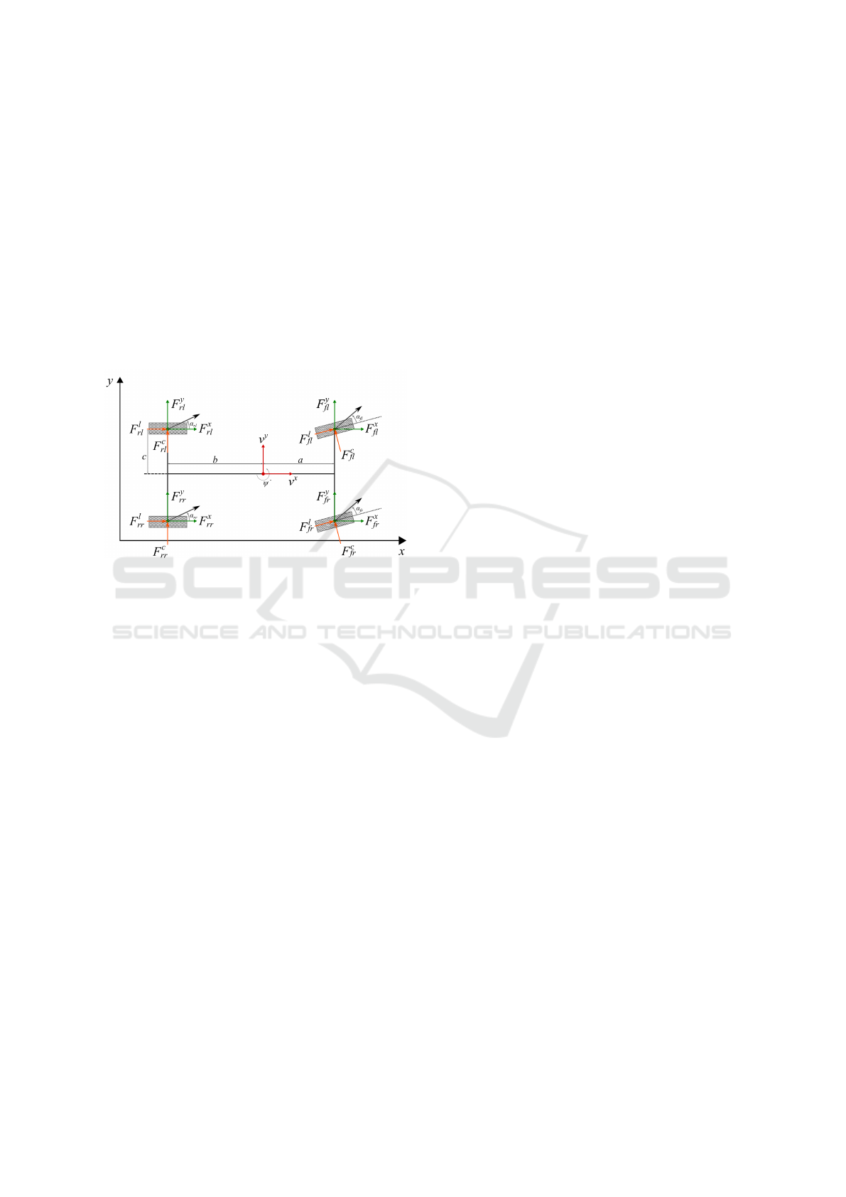
For the analytical car model we used a 4 wheel model

presented in Fig. 1 which was also used in some pre-

vious works (Buyval et al., 2017) (Frasch et al., 2013).

The chassis dynamic equations used in this paper are

presented in (1a)-(1e)

Model Predictive Path Integral Control for Car Driving with Dynamic Cost Map

249

m ˙v

= F

f r

+ F

f l

+ F

+ mv

ψ, (1a)

m ˙v

= F

f r

+ F

f l

+ F

− mv

ψ, (1b)

ψ =a(F

f l

+ F

f r

) − b(F

+ F

)

+ c(F

f r

− F

f l

+ F

− F

(1c)

˙x = v

cosψ − v

sinψ, (1d)

˙y = v

sinψ + v

cosψ, (1e)

where m denotes the mass and I

the moment of in-

ertia of the car. The geometric parameters of the car

are characterized by a, b and c, in Fig. 1. The compo-

nents of the tire contact forces are denoted by F

and

Figure 1: The 4-wheel vehicle model in inertial coordinates.

As opposed to the model presented by (Frasch

et al., 2013) we decided to avoid modelling of the

wheel rotation dynamics. That was done to improve

the computational efﬁciency. For the same reason, we

utilized Pasejka’s magic formula only for estimating

lateral tire forces. Also, we decided to exclude the

engine and the transmission and only account them

together as a torque force.

The equation for the calculation of longitudinal

tire forces is presented in (2).

= F

∗ D

/4 (2)

where F

is the traction force produced by the engine

or brakes, C

and C

are parameters of rolling and air

resistance forces respectively. D

traction distribution

factor for each wheel.

Also in comparison with papers (Buyval et al.,

2017) (Frasch et al., 2013) papers we did not modify

the time-dependent model into the track-dependent

one, because in MPPI algorithm this allows us es-

timating trajectories with a cost map which is more

convenient. In addition, this gives the ability to ac-

count dynamics of the vehicle and its surroundings in

a more comfortable time-depended form.

3.2 Suspension Model

To get all of the advantages of the 4 wheel chassis mo-

del it is needed to consider the weight transfer across

different wheels while performing turns. In our pre-

vious work (Buyval et al., 2017) we utilized algebraic

expressions, describing the weight transport as with

respect to linear and angular speeds of the car. Howe-

ver, this approach does not allow to consider suspen-

sion dynamics.

In this work we used the model of lateral rolling

with one degree of freedom which was presented by

(Rajamani, 2011). For this reason into the system of

equations (1) two additional state variables were ad-

ded: φ - rolling angle and

φ - angular speed of rolling.

The equation for estimation of the angular speed of

rolling is showed in (3)

+ mh

)

φ = ma

cos(φ) + mgh

sin(φ)

−0.5k

sin(φ) − 0.5b

φcos(φ)

(3)

where I

is the roll moment inertia around center of

gravity, m is the total vehicle mass, l

is the distance

between the left and the right suspension locations, a

is the lateral acceleration experienced by the vehicle,

is the height of the c.g. of the sprung mass from the

roll center, b

is the suspension damping coefﬁcient

and k

is the suspension stiffness.

Despite the fact that additional state variables in-

crease the computational time of the model, they do

not increase the approximation of the real object, but

also give the ability to use the estimated rolling an-

gle in the object function of the MPPI algorithm. It is

especially important for vehicles with soft suspension

and a hight center of gravity.

4 DYNAMIC COST MAP

One of the critical components of the object function

which is optimized by MPPI is a cost of the path along

the estimated trajectory. This cost is formed based on

sum of costs present at each particular point along a

trajectory which is obtained from cost map.

Paper (Williams et al., 2016) describes the appro-

ach utilizing a statically generated cost map corre-

sponding to a priori known track conﬁguration. Aut-

hors of (Drews et al., 2017) offer using a convolution

neural network to build a cost map based on camera

images. Both works consider the cost map to be static

within one iteration of MPPI even if it contains dyna-

mic objects.

Dynamic cost map that we suggest using in this

work assumes that during the trajectory sampling the

ICINCO 2018 - 15th International Conference on Informatics in Control, Automation and Robotics

250

algorithm should move dynamic obstacles after each

sampling step. Fig. 2 shows the comparison of several

MPPI trajectory sampling steps in the case of static

and dynamic cost map usage.

On the presented ﬁgure in the case when the sta-

tic cost map is used the red car plans an overcoming

maneuver at the end of the trajectory because it assu-

mes blue car to be there. But in a real situation at the

moment of time when the red car reaches the point

the blue car will be gone ahead. In addition, there

may be cases when MPPI may fail to ﬁnd the solution

using static cost map. For example, while moving al-

ong the tight road, where overcoming is not possible

the MPPI will not ﬁnd a solution if there will be a car

moving ahead of the object car.

The main difﬁculty of the algorithm implementa-

tion is a constraint of keeping relatively good time

performance. A sampling of each particular trajec-

tory is done on a separate CUDA core, which allows

to provide pretty good amount of concurrently sam-

pled trajectories. In addition, all operations referred

to trajectory’s cost estimation are done in GPU me-

mory. So cost map update related to dynamic ob-

stacles should be done in between sampling steps in

GPU memory too. Also, it is needed to be considered

that the size of cost map may be pretty big so upda-

ting it with one GPU core may be slow. This creates

a bottle neck where estimated by separate cores tra-

jectories will have to wait for one GPU core to update

the map. For that reason, we have implemented con-

current map update. That was done via binding of

each particular dynamic object with a separate GPU

core. So each thread should update only cost map’s

part related to the bound object. If dynamic objects

are absent in the current moment of time than no re-

sources are spent on updating the map.

5 SIMULATION EXPERIMENTS

To proof the workability of the described approach

we used the simulator based on Unity engine. It al-

lows us to model the car dynamics with a high preci-

sion including such components as transmission, bra-

king system and tires. In addition, simulator gives the

opportunity to model a variety of sensors: lidars, ra-

dars, GPS and IMU. The algorithm was implemented

in ROS framework. Utilizing ROS allowed us to make

debugging and logging easier. All simulation results

were obtained on a PC with the following specs: Intel

i7-7700 CPU at 2.8GHz with NVIDIA GeForce GTX

1050 Ti 4GB under Ubuntu 16.0 and ROS Kinetic.

All experiments were done using a car with follo-

wing parameters: m = 1000kg, I

= 600kgm

, a =

1.68m, b = 1.35m, c = 0.7m. Length of planning ho-

rizon is equal to 50 steps and control rate is 20 Hz for

all cases.

We have conducted 3 experiments to demonstrate

the efﬁciency of presented method: (I) bypass of a sta-

tic obstacle with lane changing (considering the dy-

namics of other cars) (II) overcoming of a bus with

driving in the oncoming lane considering oncoming

cars (III) intersection crossing with giving a way to

vehicles moving along main road.

In the ﬁrst experiment, the controlled car is loca-

ted in a right lane of the road in an initial moment of

time. On the left lane, there are 3 buses moving in

the same direction with a speed of 10 m/s. Approxi-

mately, after 150 meters on right lane roadworks are

taking place. For this reason, the algorithm should

plan to get around this obstacle with consideration of

buses on the neighbor lane. The trajectory obtained

during this experiment is presented in Fig. 3

In the second experiment, the object car was mo-

ving along the right lane behind the bus that was mo-

ving at a constant speed of 10 m/s. On the oncoming

lane in opposite direction, 2 buses are moving with

the same constant speed. Trajectory obtained in this

experiment is represented in Fig. 4

In the third experiment the car was moving to-

wards the crossing where it had to give the road to 3

buses moving from left direction along the main road.

On all three ﬁgures the trajectory of the car con-

trolled by MPPI is shown as a gradient line with co-

lor denoting the current speed. Sampled positions of

buses are represented with triangles of different co-

lors. Numbers along the trajectory represent same

moments of time. Fig. 6 represents the example of

road conditions modeled in Unity simulation environ-

ment.

To estimate the efﬁciency of the algorithm while

estimating different numbers of trajectories we used

a basic scenario of overcoming the bus moving for-

ward with a speed of 10 m/s. While experimenting

the time required to travel 250 meters and overcome

the bus was estimated. in addition, the quality of con-

trol was visually judged. Table 1 represents the re-

sults of execution of this experiment with a different

number of generated trajectories. We can see from

the table 1 that the execution of one iteration almost

not increasing with the growth of the number of the

trajectories. That is deﬁnitely a merit of concurrent

estimation run on separate NVidia GPU cores. The

total time of an overcoming maneuver on 250 meter

distance also does not change signiﬁcantly. However,

with a decrease of the generated trajectories the qua-

lity of the control was getting worse. In general, that

could be observed as a presence of steering control

Model Predictive Path Integral Control for Car Driving with Dynamic Cost Map

251

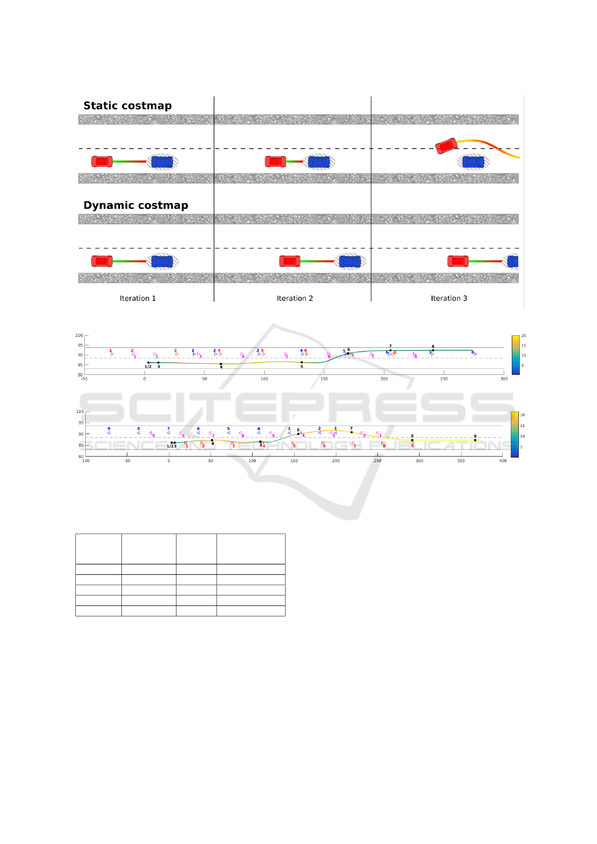
Figure 2: Comparison of static and dynamic cost maps.

Figure 3: Trajectory of the car in experiment of avoiding static obstacle and lane changing.

Figure 4: Trajectory of the car in experiment with bus overcoming.

Table 1: Iteration time, maneuver execution time for diffe-

rent number of trajectories.

Number

of trajec-

tories

Iteration

time, ms

Exec.

time, s

Quality control

512 13.6 15.1 Some oscillations

1024 14.1 14.85 Some oscillations

2048 15.3 14.9 Stable

4096 16.5 14.9 Stable

8192 19.3 14.85 Very stable

oscillations.

Trajectories of the car and other dynamic objects

with time marks and speeds. Table of MPPI stages

execution time distribution

The video of all three experiments is availa-

ble through the following link: https://youtu.be/

9FY93a2lq28.

6 CONCLUSION

This work presents the extension to the MPPI algo-

rithm which allows to plan the trajectory and cont-

rol signals for an autonomous car in a dynamic envi-

ronment considering relative surrounding object mo-

vement. The cost map update and the core algorithm

MPPI are implemented as concurrent processes on

NVidia multi-core graphics processing unit. This in-

sures the 50Hz control rate. The straightforward mat-

hematical model was used to describe a car as a sy-

stem under control, allowing to use the algorithm on

different cars only by changing parameters. Unity

was used to carry out simulation experiments aided

to test and proof the developed algorithm.

For the future plans, authors think of extending

the cost map synthesis procedure with data acquired

from cameras and 3D lidar. Also it is planned to fuse

a priori knowledge about road maps with data from

ICINCO 2018 - 15th International Conference on Informatics in Control, Automation and Robotics

252

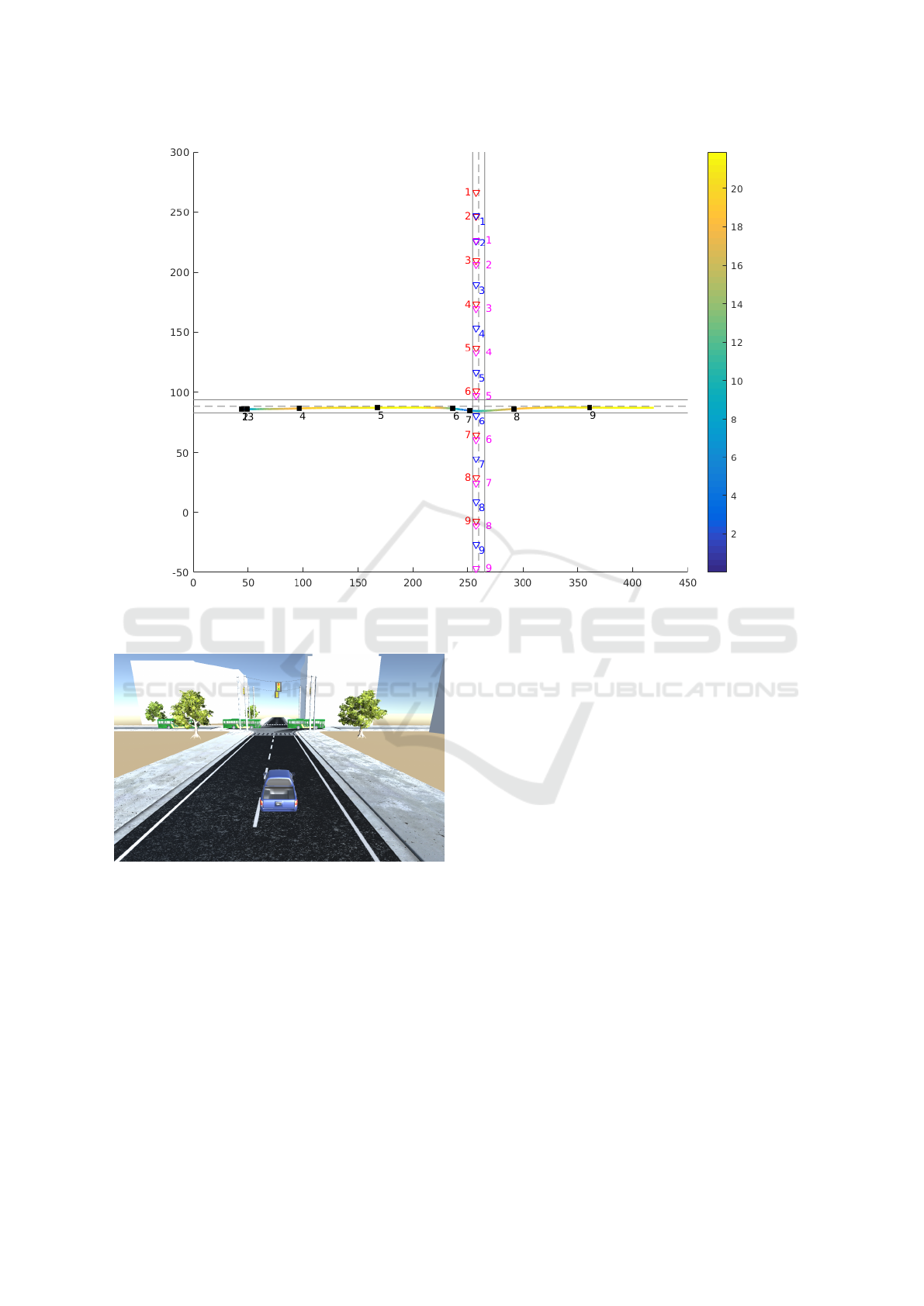
Figure 5: Trajectory of the controlled car obtained during passing road crossing.

Figure 6: An example of intersection crossing in simulation

environment.

sensors. In addition, we think of testing this approach

on a truck and a car equipped with relevant sensors

and actuators.

ACKNOWLEDGEMENTS

This research has been supported by the Russian

Ministry of Education and Science within the Fe-

deral Target Program grant (research grant ID RF-

MEFI60917X0100).

REFERENCES

Bojarski, M., Del Testa, D., Dworakowski, D., Firner, B.,

Flepp, B., Goyal, P., Jackel, L. D., Monfort, M., Mul-

ler, U., Zhang, J., et al. (2016). End to end learning for

self-driving cars. arXiv preprint arXiv:1604.07316.

Bojarski, M., Yeres, P., Choromanska, A., Choromanski,

K., Firner, B., Jackel, L., and Muller, U. (2017).

Explaining how a deep neural network trained with

end-to-end learning steers a car. arXiv preprint

arXiv:1704.07911.

Buyval, A., Gabdulin, A., Mustaﬁn, R., and Shimchik,

I. (2017). Deriving overtaking strategy from nonli-

near model predictive control for a race car. In 2017

IEEE/RSJ International Conference on Intelligent Ro-

bots and Systems (IROS), pages 2623–2628.

Drews, P., Williams, G., Goldfain, B., Theodorou, E. A.,

and Rehg, J. M. (2017). Aggressive deep driving: Mo-

del predictive control with a cnn cost model. arXiv

preprint arXiv:1707.05303.

Frasch, J. V., Gray, A., Zanon, M., Ferreau, H. J., Sager, S.,

Borrelli, F., and Diehl, M. (2013). An auto-generated

nonlinear mpc algorithm for real-time obstacle avoi-

dance of ground vehicles. In 2013 European Control

Conference (ECC), pages 4136–4141.

Kappen, H. J. (2005). Linear theory for control of non-

linear stochastic systems. Physical review letters,

95(20):200201.

Model Predictive Path Integral Control for Car Driving with Dynamic Cost Map

253

Rajamani, R. (2011). Vehicle dynamics and control. Sprin-

ger Science & Business Media.

Verschueren, R., Bruyne, S. D., Zanon, M., Frasch, J. V.,

and Diehl, M. (2014). Towards time-optimal race car

driving using nonlinear mpc in real-time. In 53rd

IEEE Conference on Decision and Control, pages

2505–2510.

Williams, G., Aldrich, A., and Theodorou, E. (2015).

Model predictive path integral control using covari-

ance variable importance sampling. arXiv preprint

arXiv:1509.01149.

Williams, G., Aldrich, A., and Theodorou, E. A. (2017a).

Model predictive path integral control: From theory to

parallel computation. Journal of Guidance, Control,

and Dynamics, 40(2):344–357.

Williams, G., Drews, P., Goldfain, B., Rehg, J. M., and The-

odorou, E. A. (2016). Aggressive driving with model

predictive path integral control. In Robotics and Auto-

mation (ICRA), 2016 IEEE International Conference

on, pages 1433–1440. IEEE.

Williams, G., Wagener, N., Goldfain, B., Drews, P., Rehg,

J. M., Boots, B., and Theodorou, E. A. (2017b). Infor-

mation theoretic mpc for model-based reinforcement

learning. In Robotics and Automation (ICRA), 2017

IEEE International Conference on, pages 1714–1721.

IEEE.

ICINCO 2018 - 15th International Conference on Informatics in Control, Automation and Robotics

254