The Feasibility and Effectiveness of P300 Responses using Low

Fidelity Equipment in Three Distinctive Environments

Patrick Schembri, Richard Anthony and Mariusz Pelc

Department of Computing and Information Systems, University of Greenwich, Greenwich London, U.K.

Keywords: Brain Computer Interface (BCI), Electroencephalography (EEG), Event-Related Potential, P300 Speller.

Abstract: In this paper we investigate the viability, practicability and efficacy of eliciting P300 responses based on the

P300 speller BCI paradigm (oddball) and the xDAWN algorithm, with five healthy subjects; while using a

non-invasive Brain Computer Interface (BCI) based on low fidelity electroencephalographic (EEG)

equipment. The experiments were performed in three distinctive environments: lab conditions, mild and

controlled user distractions, and real world environment (realistic sound and visual distractions present).

Our main contribution is the assessment of the ways and extents to which different degrees of user

distraction affect the detection success achievable using low fidelity equipment. Our results demonstrate the

applicability of using off-the-shelf equipment as a means to successfully and effectively detect P300

responses, with different degrees of success across the three distinctive types of environment.

1 INTRODUCTION

In this paper we investigate the ability, practicability

and efficacy of eliciting P300 responses using low

fidelity equipment in three distinctive environments;

lab conditions, mild and controlled user distractions

and real world environment. Our research makes use

of a non-invasive Brain Computer Interface (BCI)

on the basis of Electroencephalography (EEG). The

work presented here is part of a larger EEG based

project and in continuation of our previous papers

(Schembri et al., 2017) (Schembri et al., 2018).

One of the main type of signals utilized in EEG,

are the Evoked Potentials (EP) / Evoked Responses

(ER) and/or Event-related Potentials (ERP). In

general and for the purpose of this paper we will

henceforth refer to these as Event-related Potentials

(ERP) even though ERPs are considered the

successors of EP where a set of robust potentials

where identified to reflect higher order brain

processing (Runehov et al., 2013). However in the

scientific community these terms are commonly

used interchangeably.

ERPs are slow voltage fluctuations or electrical

potential shifts recorded from the nervous system.

These are time-locked to perceptual events

following a presentation of a stimulus being either

cognitive, sensor or motor stimuli. The term time-

locked implies that the time between the event and

voltage fluctuation is relatively constant; for

instance the P300 component is a positive wave that

can appear anywhere from 300 to 800ms after the

response (Stern et al., 2001). The major drawback of

ERP is that its signal-to-noise ratio is typically quite

low (Stern et al., 2001) (Ding and Ye, 2004) and

signal averaging over a number of trials is required.

ERP components are predominantly classified as

either exogenous (reliant on the external stimulus

characteristics) or endogenous (dependent on the

subjects actions and intentions); however this should

be considered as a dimension rather than a rigorous

classification (Ward, 2015) (Näätänen, 1992).

One of the most renowned ERP components is

the aforementioned P300 (P3), which was first

described by Sutton (Sutton et al., 1965) and has

been used in a multitude of paradigms. The most

prominent paradigm; the P300 speller BCI

paradigm; was originally described by (Farwell and

Donchin, 1988), where alphanumeric characters or

1-word commands, 36 in total, are presented in a six

by six grid as depicted in Figure 1 (the term symbol

will refer to any alphanumeric character in this

figure). The methodology used derives from the

oddball paradigm; first used in ERPs by Nancy,

Kenneth and Steven (Squires et al., 1975) where the

subject is asked to distinguish between a common

stimulus (nontarget) and a rare stimulus (target). In

Schembri, P., Anthony, R. and Pelc, M.

The Feasibility and Effectiveness of P300 Responses using Low Fidelity Equipment in Three Distinctive Environments.

DOI: 10.5220/0006895000770086

In Proceedings of the 5th International Conference on Physiological Computing Systems (PhyCS 2018), pages 77-86

ISBN: 978-989-758-329-2

addition and unless otherwise noted in this paper, the

P300 will always refer to the P300b (P3b) which is

elicited by task relevant stimuli in the centro-

parietal, rather than P300a (P3a) which is related to

automatic detection of novelty and is task irrelevant,

detected in the fronto-central.

In this paper we report a study where five

healthy subjects used a variation of Farwell and

Donchin P300 speller paradigm; where we based the

methodology on the xDAWN algorithm (Rivet et al.,

2009); to communicate nine alphanumeric characters

in three distinctive environments, while using

specific low fidelity equipment. Our aim is to assess

the effects of the disturbances on the P300 signal

and also on the signal detection accuracy.

2 EXPERIMENTAL

METHODOLOGY

The work presented in this paper will make use of

Farwell and Donchin’s P300 speller which uses

visual stimuli, where each row and column of the

spelling grid is augmented in a random order. The

subject is asked to focus on the desired symbol

(target) and mentally count (to heighten ERP) the

number of times the row and column comprising the

desired symbol is augmented. As a result of the

(target) stimuli, an exogenous and spontaneous ERP

potential known as P300; which is a positive

deviation around 300ms after the stimuli; is evoked

in the brain. The desired symbol is determined and

predicted by the intersection of the (target) row and

column. This prediction entails distinguishing

between non-target i.e. rows/columns stimuli that

does not generate a P300 component and target i.e.

row/column stimuli that generate a P300 component.

Figure 1: BCI “P300 Speller”. The screen as shown to the

subjects with the 3

row highlighted.

In any recorded EEG signal, the P300 component

which has a typical peak potential between 5-10µV

(Peters and Skowron, 2006), is embedded and

masked by other brain activities (typical EEG signal

+-100µV) such as muscular and/or ocular artefacts

(Schembri et al., 2017) leading to a very low Signal-

to-Noise Ratio (SNR) of the P300 component. This

indicates that it would be very difficult to detect the

target stimuli from a single trial, which is denoted by

a series of augmentation, in random order, of each of

the six rows and six columns in our matrix (i.e.

twelve augmentations per trial). A popular way to

address the limited SNR of EEG is for each symbol

to be spelled numerous consecutive times and the

respective column/row epochs be averaged over a

number of trials, thus cancelling components

unrelated to stimulus onset (Wittevrongel and Van

Hulle, 2016). A trade-off exists between increasing

the number of trials per symbol (increases

classification accuracy) and the number of symbols

spelled per minute.

Apart from using low fidelity equipment, our

experiments were performed in three distinctive

environments which are explained in detail below.

Lab Conditions: the experiments were performed

in a sound-attenuated and air conditioned room.

There were no distractions;

Mild and Controlled User Distractions: the

experiments were also performed in a sound-

attenuated and air conditioned room. The following

distractions were introduced throughout the

experiment: (1) a low volume radio; (2) the

researcher walked around the subject in a methodical

way however there were no vocal interactions;

Real World Environment: the experiments were

performed in an air conditioned room. The following

distractions were introduced: (1) the room was not

sound-attenuated, it had an open window leading

onto the street and the internal door was kept open;

(2) the same low volume radio used in the mild

environment was kept running; (3) a television set

was set-up in the room and a movie was played with

medium volume; (4) the researcher walked around

the subject unsystematically, throughout the whole

experiment; (5) the researcher asked the subject two

questions: (a) what is the date of birth of your

father? and (b) what is the total of 55 + 12?; and the

subject replied. While replying the subject did not

make eye contact with the researcher and kept his

focus on the desired symbol. A note was taken

which target symbol was being spelled at the time

the questions were asked.

The training session (refer to Section 2.4) was

always performed in lab conditions.

The P300 speller was chosen for this study as our

application domain since it gave us a well-structured

defined and documented set of experiments i.e. a

PhyCS 2018 - 5th International Conference on Physiological Computing Systems

structured experimental mechanism which is

repeatable. Since using this equipment in non-lab

conditions is a novel area of research, it was decided

that P300 was a good basis for its institution due to it

being an exogenous signal i.e. a stereotypical

response, which can be produced without training.

2.1 The xDAWN Spatial Filter

The xDAWN process of spatial filtering is (1) a

dimensionally reduction method that creates a subset

of pseudo-channels (referred to as output channels)

by a linear combination of the original channels and

(2) it promotes the appealing part of the signal, such

as ERPs, with respect to the noise. This is applied to

the data before performing any classification such as

LDA (Linear Discriminant Analysis) which was

used in this paper. From an abstract point of view

the xDAWN algorithm can be divided into (1) a

least square estimation of the evoked responses and

(2) a generalized Rayleigh quotient to estimate a set

of spatial filters that maximize the SSNR.

The following is adapted from (Rivet et al.,

2009) and (Woehrle et al., 2015). Let X ∈ ℝ

S x C

the EEG data that contain ERPs and noise, with S

samples and C channels. Let A ∈ ℝ

E x C

be the matrix

of ERP signals, while E is the number of temporal

samples of the ERP (typically, E is chosen to

correspond to 600 ms or 1 s). Let N ∈ ℝ

S x C

be the

noise matrix which contains normally distributed

noise. The ERPs position in the data is given by a

Toeplitx matrix D ∈ ℝ

E x S

. The data model is given

by X = D

A+N. A is estimated by a least square

estimate using a matrix inverse (pseudoinverse) as

shown in formula (1).

Â=min



=|| − ||



(





)









(1)

Let W ∈ ℝ

S x F

be the pseudo-channels while F

represents the filters for projection. The result is the

filtered data matrix X

= XW. According to (Rivet et

al., 2009), the optimal filters W can be found by

maximizing the SSNR as given by the generalized

Rayleigh quotient:

Ŵ=max



(







Â)

(







)

(2)

The optimization problem is solved by

combining a QRD (QR matrix decomposition) with

an SVD (singular value decomposition). A more

thorough explanation is found at (Rivet et al., 2009).

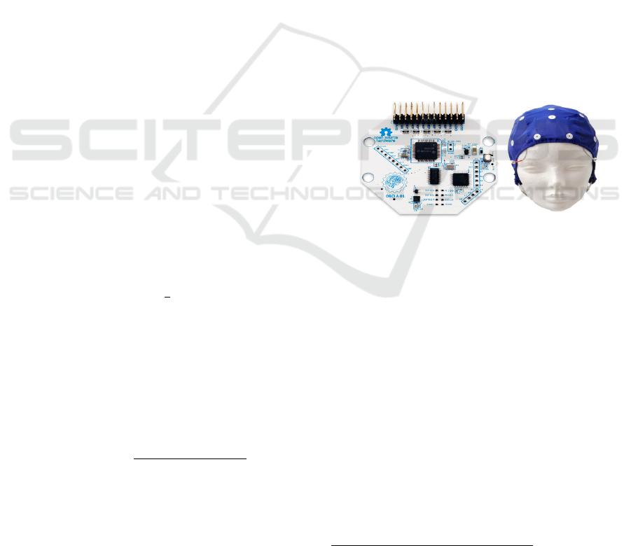
2.2 Equipment Used

The work reported herein is based on an OpenBCI

32-bit board (called Cyton) connected with an

Electro-Cap using the international 10/20 system for

scalp electrode placement in the context of EEG

experiments. This is illustrated in Figure 2.

The Cyton board’s microcontroller is the

PIC32MX250F128B with a 32-bit processor and a

maximum speed of 50MHz; storage of 32KB of

memory and is Arduino compatible. The board uses

the ADS1299 IC developed by Texas Instruments,

which is an 8-Channel, 24-Bit, simultaneous

sampling delta-sigma, Analogue-to-Digital

Converter used for bio potential measurements. The

system comes with a pre-programmed USB dongle

for wireless communication which communicates

with the low cost RFDuino RFD22301

microcontroller built on the OpenBCI board. An

additional feature which is included in the OpenBCI

board is a 3-axis accelerometer from ST with model

LIS3DH. A more thorough explanation of the

hardware components of the Cyton can be found in

our previous paper

(Schembri et al., 2017).

Figure 2: Cyton Board and Electro-CAP.

The Electro-Cap being used in our experiments

has the fabric which is made from elastic spandex

and has recessed pure tin wet electrodes directly

attached to the fabric. The term wet electrodes type,

implies that the use of an electrolyte gel is required

to make effective contact with the scalp; otherwise it

may result in impedance instability

2.3 Subjects

We enlisted five healthy subjects, three males and

two females, aged 29-38 which voluntarily

participated in this study. Four of the five subjects’

native language was Maltese and the fifth subject’s

native language was English. All subjects spoke

fluent English and were familiar with the symbols

displayed on our screen as depicted in Figure 1. One

http://www.scitepress.org/DigitalLibrary/PublicationsDet

ail.aspx?ID=OKHKQwhPuUs=&t=1

The Feasibility and Effectiveness of P300 Responses using Low Fidelity Equipment in Three Distinctive Environments

of the subjects had previous experience using BCI

and the P300 speller and will henceforth be referred

as subject3 in the results (refer to Section 3). The

other four subjects had never used or performed any

BCI, nor have they ever seen a P300 speller.

Three other subjects that assisted in the initial

experimentation phase where we assessed the

viability of our equipment with the P300 component;

however they did not take part in the official

experiments and hence aren’t included in the results.

2.4 Experimental Procedure and

Stimuli

The EEG signals where sampled at 250Hz, while the

sampling precision was 24-bit. The recordings were

stored anonymously as raw data in OpenVIBE .ov

format. These were later converted to a comma

separated value (csv) files for offline analysis. Eight

EEG electrodes where used in different regions of

the scalp according to the International 10-20

System. The equipment we are using supports a

maximum of sixteen electrodes. The Cyton board

supports eight electrodes and an extension module

(called Daisy) supports an additional eight

electrodes. After initial analysis we did not see a

major improvement between eight and sixteen

electrodes and we have opted to exclude the use of

the daisy module, hence the extra eight electrodes.

The electrode positions C3, Cz, C4, P3, Pz, P4,

O1 and O2 were selected. This is because the spatial

amplitude dispersal of the P300 component is

symmetric around Cz and its electrical potential is

maximal in the midline region (Cz, Pz) (Ogura et al.,

1995) as shown in Figure 3. It typically increases in

magnitude from the frontal/occipital to parietal lobes

(Johnson, 1993). The midline region is still widely

used in almost all papers related to P300 detection

such as (Venuto et al., 2017) and (Frey, 2016).

Figure 3: P300 Amplitude Dispersal – from BCI2000.org.

A referential montage was selected with the

reference electrode being placed on the left earlobe

A1 given that, in general, a mastoid or earlobe

reference will produce a robust P300 response. The

right ear lobe A2 is used as ground. The electrodes

are referenced to electrode A1 as follows: Ch1: C3;

Ch2: Cz; Ch3: C4; Ch4: P3; Ch5: Pz; Ch6: P4; Ch7:

O1; Ch8: O2 as shown in Figure 4. Nonetheless and

if required other types of montage can be

reconstructed from the chosen montage by executing

a simple mathematical operation (re-referencing) in

the “offline” analysis, as explained in our previous

paper (Schembri et al., 2017).

Figure 4: Electrode placement following the 10-20 system.

In the induction session, each subject was briefed

on the hardware being used and was shown a

demonstration of an online P300 speller.

Subsequently, the subjects’ were informed on the

following: (1) they would be performing the same

experiment four consecutive times; in the training

phase; in lab conditions; with mild distractions; and

in a real world environment, (2) the symbols to spell

were “P3SPELLER” respectively, (3) there might be

some distractions and that they are an integral part of

the experiment, (4) they should answer any

questions asked throughout the experiments while

trying to maintain focus on the desired symbol. Any

subjects’ query was answered at this stage.

Before the start of the experiments, each subject

was asked to relax for a few minutes in a seated

position. The subject was seated approximately one

meter away from the display. The researcher and his

equipment were situated on the left side of the

subject. The experiment was started when the

subject was able to properly perform the task at hand

and had no additional questions. Prior to the start of

every experiment, the electrodes impedance was

confirmed to be less than 5KΩ.

The display presented to the subjects is shown in

Figure 1 where 36 symbols were presented in a 6x6

matrix. The subjects’ task was to visually focus their

attention on the requested symbol, which was

preceded by a cue i.e. one of the symbols was

highlighted in blue at the beginning of the trials as

depicted in Figure 5. The subject was asked to count

the number of times the required symbol flashed

which is then determined and predicted by the

intersection of the (target) row and column. This

PhyCS 2018 - 5th International Conference on Physiological Computing Systems

prediction entails distinguishing between non-target

i.e. rows/columns stimuli that does not generate a

P300 component and target i.e. row/column stimuli

that generate a P300 component. Each row and

column in the matrix was augmented randomly for

100ms and the delay between two successive

augmentations was 80ms. This led to an

interstimulus interval (ISI) of 180ms. For each

symbol, six rows and six columns were augmented

for fifteen repetitions and there was no inter-

repetition delay. However there was a 3s inter-trial

period between the end of the trials of one symbol

and the beginning of trials of the next symbol. This

allowed the subject to focus the attention on the next

symbol. At the end of each symbol run, the predicted

symbol was highlighted in green which indicated

whether the subject got the correct target symbol as

depicted in Figure 5. The subjects were given a short

break between experiments.

Figure 5: Requested symbol highlighted in blue and, after

trials, predicted symbol highlighted in green.

The training phase consisted of one session with

15 random symbols by 15 trials each (i.e. 12 flashes

of columns/rows per trial * 15 trials = 180 flashes

per symbol). This was done in lab conditions and

without any distractions. In previous experiments

with different subjects we have seen that there was

no discernible difference in further increasing the

number of trials per symbol or number of symbols,

in the training phase. According to previous success

in the usability of the P300 speller with low cost

equipment such as (Frey, 2016); two criteria were

established to evaluate the optimal number of

symbols and trials in the training session which

correspond to two desired accuracies of 80% - 90%

in an online system in lab conditions. The recording

of the training phase took approximately 9 minutes.

The Lab Conditions, Mild and Controlled User

Distractions and Real World Environment consisted

of one session each with the aforementioned

conditions and configurations while spelling the

symbols “P3SPELLER” consecutively. Similarly to

the training phase, each symbol had fifteen trials

each. The recording of each environment session

lasted approximately 6 minutes.

In total, there were 15 symbols spelled in the

training phase and 9 symbols spelled in each of the

three environments per subject. Hence due to the

matrix disposition there were in total 2700 flashes in

the training phase, amongst which 450 were targets;

and 1620 flashes in each environment (1620 * 3

environments), amongst which 270 (270 * 3

environments) were targets. These values are per

subject. The data was stored anonymously by

referring to the subjects as subject1-5 respectively.

2.5 Signal Processing - Online

The signal was acquired using OpenViBE 2.0.0

which is a C++ based software platform designed for

real-time processing of biosignal data. Its most

distinguishable feature is its graphical language for

designing signal processing chains and its main

components include the acquisition server and the

designer. The acquisition server interfaces with the

Cyton board and generates a standardized signal

stream that is sent to the designer which in turn is

used to construct and execute signal processing

chains stored inside scenarios.

The signal was obtained via the acquisition

server which does not communicate directly with the

Cyton board. Instead it provides a specific and

dedicated set of drivers that does this task. The

signal was obtained at a sampling rate of 250Hz with

8 EEG and 3 accelerometer (auxiliary) channels.

The sample count per sent block was set to 32 which

define how many samples should be sent per

acquired channel in a single buffer with valid values

being powers-of-two, from 2

to 2

. The board reply

reading timeout was set to 5000ms and the flushing

timeout was set to 500ms. The drift tolerance was

set to 20ms, even though OpenVibe version 2.0

largely relies on TCP tagging to align stimulation

markers to the EEG signal; which we have used in

our experiments. The drift correction can introduce

artefacts in the signal and mask other potential faults

such as a driver bug; which however did not occur in

our experiments. Nevertheless this makes the drift

correction mechanism redundant and its use will be

discontinued in future ERP papers. The experiment

paradigm was controlled by the designer where a

number of scenarios were executed in succession.

The first scenario was the acquisition of the

signal and stimuli markers for the training phase.

The recordings included the raw EEG and stimuli.

The second scenario entailed the pre-processing

of the signal where it trained the spatial filter using

the xDAWN algorithm. The subjects’ data recorded

in the training session was utilized, with the

The Feasibility and Effectiveness of P300 Responses using Low Fidelity Equipment in Three Distinctive Environments

following configuration and modalities. Initially we

have chosen to eliminate the last three auxiliary

channels which stored the auxiliary data of the

accelerometer since the board was firmly placed on

the desk and this information was not required.

Subsequently a Butterworth band pass filter of 1Hz-

20Hz was applied with an order of 5 and a ripple

(dB) of 0.5 to remove the DC offset, the 50Hz (60Hz

in some countries) electrical interference, any signal

harmonics and unnecessary frequencies which are

not beneficial in our experiments. Next, no signal

decimation was used since the sampling rate and

count per buffer previously used in the acquisition

server were not compatible with the actual signal

decimation factor due to the Cyton board’s sampling

rate of 250Hz (no available value in the sample

count per block is factorable with 250Hz). However

we still passed the signal through a time based

epoching which generated ‘epochs’ (signal slices)

with duration of 0.25s and time offset of 0.25s

between epochs (i.e. we created a temporal buffer to

collect the data and forward them into blocks). This

implies that there was no overlapping of data and

that the inputs for the xDAWN spatial filter and the

Stimulation based epoching were based on epochs of

0.25s rather than the whole data. In simplest terms

we had one point for every 0.25s of data which made

our signal coarser. Subsequently we passed the time

based epochs and stimulations to the Stimulation

based epoching which sliced the signal into chunks

of a desired length following a stimulation event.

This had an epoch duration of 0.6s (p300 deviation

around 0.3s after the stimuli) and no offset. Lastly,

the stimulations, time based epochs and the

stimulation based epochs were passed to the

xDAWN trainer which in simplest terms trains

spatial filters that best highlight ERPs. The xDAWN

expression, utilized in OpenVIBE, which has to be

maximized, varies marginally from the original

xDAWN (Rivet et al., 2009) formula where the

numerator includes only the average of the target

signals. In addition, the implemented algorithm

maximizes the quantity via a generalized eigenvalue

decomposition method in which the best spatial

filters are given by the eigenvectors corresponding

to the largest eigenvalues (Clerc et al., 2016). This

scenario created twenty-four coefficients values in

sequence (i.e. 8 input channels by 3 output channels)

that were used in the following scenario.

The third scenario carried on the pre-processing

of the signal where it trained the classifier, partially

with the values from the previous scenario. Once

again the subjects’ raw data which was recorded in

the training session was utilized with the elimination

of the last three aux channels, the omission of signal

decimation and the application of a Butterworth

band pass filter of 1Hz-20Hz; identical to the

previous scenario. Subsequently the parameters of

the xDAWN spatial filter that were generated in the

second scenario which include the 24 spatial filter

coefficients, 8 input channels and output 3 output

channels were used. This spatial filter generated 3

output channels from the original 8 input channels;

each output channel was a linear combination of the

input channels. The output channels were computed

by performing the “sum on i (Cij * Ii )” as shown in

formula (3), where Ii represents the input channel (n

is set to 8), Oj represents the output channel and Cij

is the coefficient of the ith input channel and jth

output channel in the spatial filter matrix.

 =  ∗ 





(3)

Subsequently the outputted signals (i.e. the 3

output channels) and the stimulations were passed

equivalently into two separate stimulation based

epoching; for the target and the non-target selection.

These had epoch duration of 0.6s and no offset. The

output i.e. both epoch signals (target and non-target)

were again separately computed with block

averaging and passed through a feature aggregator

that combined the received input features into a

feature vector that was used for the classification.

This implies that two separate feature vector streams

were outputted; the target and non-target selections.

Ultimately both vector streams and the stimulations

were passed through our classifier trainer. We have

opted to pass all the data through a single classifier

trainer, hence the native multiclass strategy was

chosen, which used the classifier training algorithm

without a pairwise strategy. The algorithm chosen

for our classifier is the regular LDA. The output at

this stage is a trained classifier with the settings

outputted to a file for use in the next scenario.

The fourth scenario consisted of the actual online

experiments and was more complex, since it was

necessary to collect data, pre-process it, classify it

and provide online feedback to the subject. The

front-end consisted of displaying the 6x6 grid,

flashing rows and columns and give feedback to the

subject. The back-end consisted of a number of

processes. Primarily, the data was acquired from the

subject in real-time and similar to what was done in

the previous scenarios, the last three aux channels

were eliminated, signal decimation was omitted, a

Butterworth band pass filter of 1Hz-20Hz was used

PhyCS 2018 - 5th International Conference on Physiological Computing Systems

and the parameters of the xDAWN spatial filter that

were generated in the second scenario which

included the twenty-four spatial filter coefficients

were used. Subsequently the output and the

stimulations were passed in the Stimulation based

epoching which had epoch duration of 0.6s and no

offset. This was then averaged and passed through a

feature aggregator to produce a feature vector for

the classifier. Lastly the classifier processor

classified the incoming feature vectors by using the

previously learned classifier (classifier trainer).

The fifth scenario allows us to replay the

experiments by selecting the raw data file and re-

processing the functions of the fourth scenario.

2.6 Signal Processing - Offline

The captured raw data was converted from the

proprietary OpenVIBE .ov extension to a more

commonly used .csv format using a particular

scenario aimed for this task. The outputs were two

files in .csv format which contained the raw data and

stimulations respectively. These were later imported

into MATLAB R2014a tables called samples and

stims and then converted to arrays. Subsequently any

unnecessary rows and columns in the samples array

were removed. These consisted of the first rows

which contained the time header, channel names and

sampling rate; the first column which contained the

time(s) and the last three columns which stored the

auxiliary data of the accelerometer. Next, we filtered

out the stims array to include the target stimulations

with code (33285); non-target stimulations (33286);

visual stimulation stop (32780), which is the start of

each flash of row or column; and segment start

(32771), which is the start of each trial (12 flashes, 6

rows and 6 columns make up 1 trial). Additional

data such as the sampleTime, samplingFreq and

channelNames variables were extracted from the

data and stored in the workspace.

The samples array was later imported into

EEGLAB for processing and for offline qualitative

and quantitative analysis. The first process was to

apply a band pass filter of 1-20HZ to eliminate the

environmental electrical interference (50Hz or 60Hz

dependent on the country), to remove any signal

harmonics and unnecessary frequencies which are

not beneficial in our experiments and to remove the

DC offset. Subsequently we import the event info

(the stimulations – stim array) in EEGLAB with the

format {latency, type, duration} in milliseconds.

Next, the imported data was used in ERPLAB

which is an add-on of EEGLAB, and is targeted for

ERP analysis. Although the dataset in EEGLAB

already contains information about all the individual

events, we have created an eventlist structure in

ERPLAB that consolidates this information and

makes it easier to access and display; and also

allows ERPLAB to add additional information

which is not present in the original EEGLAB list of

events. Subsequently we take every event we want

to average together and assign that to a specific bin

via the binlister.

Subsequently we extracted the bin-based epochs

via ERPLAB (not the EEGLAB version) and set the

time period from -0.2s before the stimulus until 0.8s

after the stimulus. We have also used baseline

correction (pre) since we wanted to subtract the

average pre-stimulus voltage from each epoch of

data. We have opted not to include any artefacts

rejection, since this was not present in our online

system. Lastly, we averaged our dataset ERPs to

produce the required results which are shown in

section 3.2.

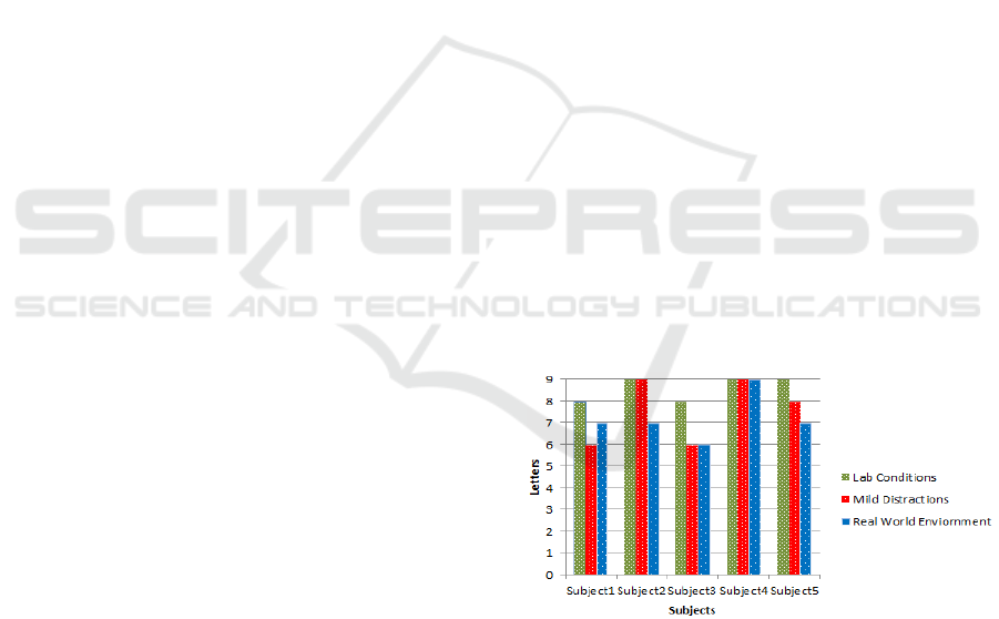
3 RESULTS

3.1 Online Analysis

Following the online experiments, we achieved the

following results per subject. The letters to be

spelled were P3SPELLER consecutively, while all

percentages shown are rounded to the nearest one.

Figure 6 depicts the results acquired per subject per

environment.

Figure 6: Graph representing the success per letter and per

subject in our three environments.

Additionally, in the following Table 1, the colour

red (bold and italic in grayscale) denotes a bad

prediction in both the row and column, the colour

blue (bold) denotes a bad prediction in the column,

while the colour purple (bold and underlined)

denotes a bad prediction in the row.

For instance, consider the following results for

Subject1 as summarized in Table 1. Lab Conditions:

The Feasibility and Effectiveness of P300 Responses using Low Fidelity Equipment in Three Distinctive Environments

the subject had an 89% success rate with the letter L

predicted as letter G i.e. the row prediction was

correct but not the column. Mild Distractions: the

subject had a 67% success rate with the letters E, L

and R predicted as Z, K and P respectively, i.e. for

the letter Z we had both row and column prediction

incorrect, while for letter K and P we had a correct

row prediction and an incorrect column prediction.

Real World: the subject had a 78% success rate with

the symbols P and L predicted as K and N

respectively. The other subject’s results follow the

same detailed description as above.

The average accuracy for all the subjects in lab

condition was 95.6%; in mild distractions it was

84.6% and in real world environment it was 80.2%.

This was in par with our hypothesis that by

increasing the distractions to the subject, the

performance of the system would be reduced. The

average accuracy per subject in all three

environments is shown in Table 2. It is interesting to

point out that the least successful subject was

subject3 which had previous experience using the

P300 speller. This is an indication that actual

training on the system doesn’t seem to affect the

performance, hence reinforcing that P300 is an

exogenous (reflex) i.e. reliant on the external

stimulus characteristics.

Table 1: Subject Results.

S Lab Conditions Mild

Distractions

Real World

Environment

S1 8 out of 9

P3SPEGLER

predicted

89% success

6 out of 9

P3SPZKLEP

Predicted

67% success

7 out of 9

P3SKENLER

predicted

78% success

S2 9 out of 9

P3SPELLER

Predicted

100% success

9 out of 9

P3SPELLER

Predicted

100% success

7 out of 9

P3SPEXFER

predicted

78% success

S3 8 out of 9

P3SPELLEF

Predicted

89% success

6 out of 9

P3SPEIIEQ

predicted

67% success

6 out of 9

P3SNDLKER

predicted

67% success

S4 9 out of 9

P3SPELLER

Predicted

100% success

9 out of 9

P3SPELLER

predicted

100% success

9 out of 9

P3SPELLER

predicted

100% success

S5 9 out of 9

P3SPELLER

predicted

100% success

8 out of 9

P3SPELL3R

predicted

89% success

7 out of 9

P3SPEILEX

Predicted

78% success

95.6% 84.6% 80.2%

Table 2: Average accuracy per subject in all environments.

S1 S2 S3 S4 S5

78%

93% 74% 100% 89%

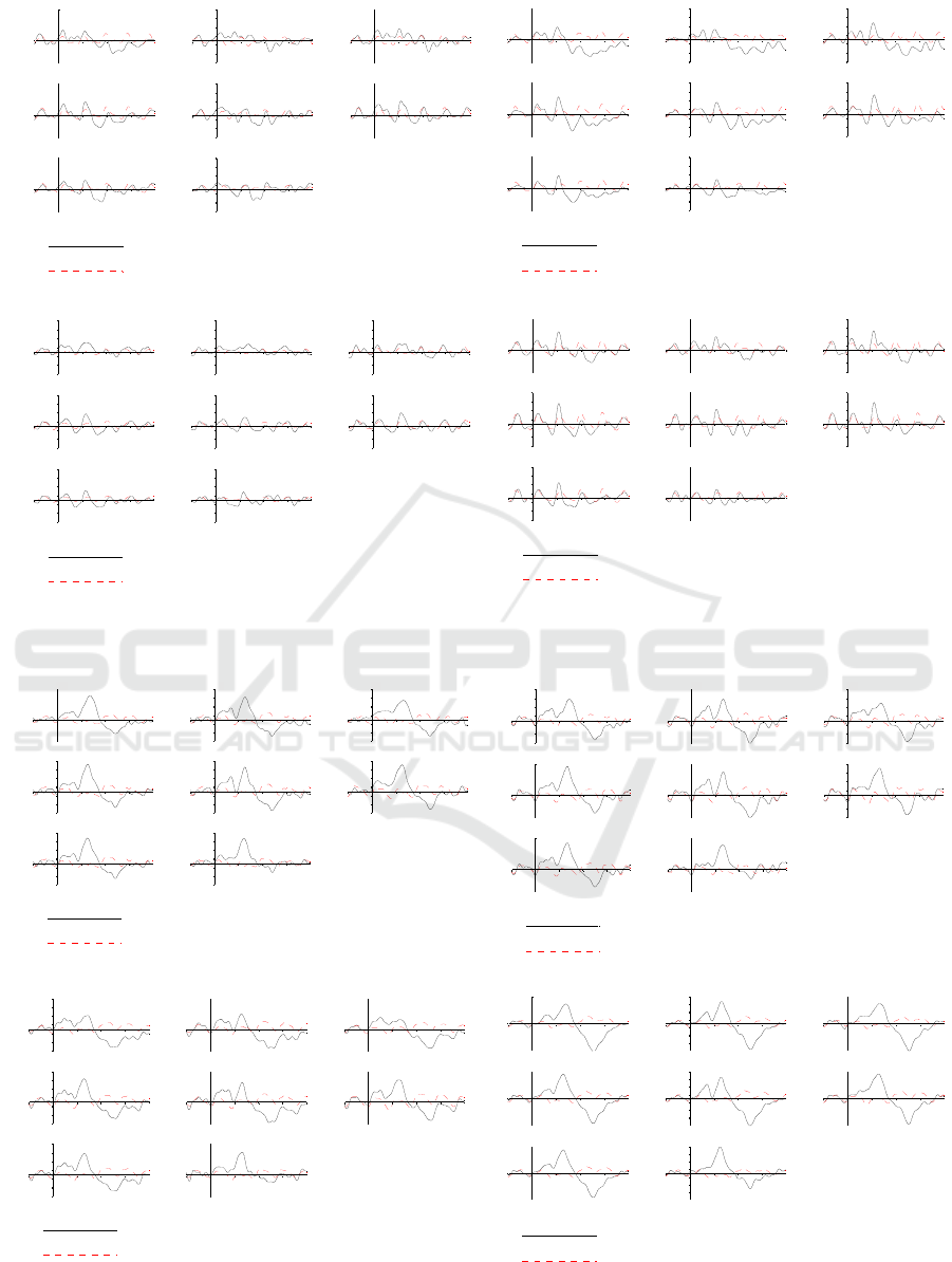
3.2 Offline Analysis

The following figures represent a sample of the

results that were processed in offline analysis. We

have chosen to show the signals of subject3 and

subject4 since they represent the lowest and highest

success rate throughout the three environments.

We have also opted to present the averaged raw

signals of every environment i.e. 9 symbols with 15

trials per symbol; with 12 flashes of columns/rows

per trial. The presented results are only passed

through a band pass filter (1-20Hz) since this is

needed to reduce the noise and unwanted

frequencies, but it does not change the P300 signal

i.e. it is essentially a pre-processing / conditioning

step, it does not contribute directly to the analysis of

the P300. In addition we have decided to refrain

from using any artefact rejection in our offline

analysis since it wasn’t present in our online system.

Furthermore we are not presenting the xDAWN

spatial filters since our aim is to show the barest raw

signal that is captured with our low fidelity

equipment within our three distinctive environments.

This work is part of a larger project where the

available data will be scrutinized in depth and results

will be published subsequently.

Figure 7(a-d) represent subject3’s lab, mild, real

world environment and training phase respectively

and similarly figure 8(a-d) represents subject4’s lab,

mild, real world environment and training phase.

4 CONCLUSION

The use of Electroencephalography (EEG) signals in

the field of Brain Computer Interface (BCI) has

gained prominence over the past decade, especially

with the institution of low cost devices, which made

it accessible to a wide variety of researchers.

However, experimentation on this technology is still

being restricted to lab conditions where the

experiments are (1) targeted for and being performed

in a noise-free environment and (2) without any

interruptions to the subject. The aim of this paper is

to steer away from perfect lab conditions and assess

to which extent our low fidelity equipment is

capable to function in a reliable and consistent

manner in the afore environments.

PhyCS 2018 - 5th International Conference on Physiological Computing Systems

a) b)

c) d)

Figure 7: Subject3’s averaged ERP over all trials in (a) lab environment (b) mild distractions and (c) real world

environment. The averaged training ERP session is shown in (d).

a) b)

c) d)

Figure 8: Subject4’s averaged ERP over all trials in (a) lab environment (b) mild distractions and (c) real world

environment. The averaged training ERP session is shown in (d).

-200 200 400 600

-5

-3

-1

-200 200 400 600

-5

-3

-1

-200 200 400 600

-5

-3

-1

-200 200 400 600

-5

-3

-1

-200 200 400 600

-5

-3

-1

-200 200 400 600

-5

-3

-1

-200 200 400 600

-5

-3

-1

-200 200 400 600

-5

-3

-1

BIN1: Target

BIN2: NonTarget

-200 200 400 600

-5

-3

-1

-200 200 400 600

-5

-3

-1

-200 200 400 600

-5

-3

-1

-200 200 400 600

-5

-3

-1

-200 200 400 600

-5

-3

-1

-200 200 400 600

-5

-3

-1

-200 200 400 600

-5

-3

-1

-200 200 400 600

-5

-3

-1

BIN1: Target

BIN2: NonTarget

-200 200 400 600

-5

-3

-1

-200 200 400 600

-5

-3

-1

-200 200 400 600

-5

-3

-1

-200 200 400 600

-5

-3

-1

-200 200 400 600

-5

-3

-1

-200 200 400 600

-5

-3

-1

-200 200 400 600

-5

-3

-1

-200 200 400 600

-5

-3

-1

BIN1: Target

BIN2: NonTarget

-200 200 400 600

-5

-3

-1

-200 200 400 600

-5

-3

-1

-200 200 400 600

-5

-3

-1

-200 200 400 600

-5

-3

-1

-200 200 400 600

-5

-3

-1

-200 200 400 600

-5

-3

-1

-200 200 400 600

-5

-3

-1

-200 200 400 600

-5

-3

-1

BIN1: Target

BIN2: NonTarget

-200 200 400 600

-5

-3

-1

-200 200 400 600

-5

-3

-1

-200 200 400 600

-5

-3

-1

-200 200 400 600

-5

-3

-1

-200 200 400 600

-5

-3

-1

-200 200 400 600

-5

-3

-1

-200 200 400 600

-5

-3

-1

-200 200 400 600

-5

-3

-1

BIN1: Target

BIN2: NonTarget

-200 200 400 600

-5

-3

-1

-200 200 400 600

-5

-3

-1

-200 200 400 600

-5

-3

-1

-200 200 400 600

-5

-3

-1

-200 200 400 600

-5

-3

-1

-200 200 400 600

-5

-3

-1

-200 200 400 600

-5

-3

-1

-200 200 400 600

-5

-3

-1

BIN1: Target

BIN2: NonTarget

-200 200 400 600

-5

-3

-1

-200 200 400 600

-5

-3

-1

-200 200 400 600

-5

-3

-1

-200 200 400 600

-5

-3

-1

-200 200 400 600

-5

-3

-1

-200 200 400 600

-5

-3

-1

-200 200 400 600

-5

-3

-1

-200 200 400 600

-5

-3

-1

BIN1: Target

BIN2: NonTarget

-200 200 400 600

-5

-3

-1

-200 200 400 600

-5

-3

-1

-200 200 400 600

-5

-3

-1

-200 200 400 600

-5

-3

-1

-200 200 400 600

-5

-3

-1

-200 200 400 600

-5

-3

-1

-200 200 400 600

-5

-3

-1

-200 200 400 600

-5

-3

-1

BIN1: Target

BIN2: NonTarget

The Feasibility and Effectiveness of P300 Responses using Low Fidelity Equipment in Three Distinctive Environments

In continuation of our previous papers (Schembri

et al., 2017) (Schembri et al., 2018) and part of this

paper’s scope; we have also resumed the validation

of our equipment’s suitability and performance,

presently, in the execution of the P300 speller

domain. We have also improved performance upon

(Frey, 2016) which was the last paper that utilized

our equipment in conjunction with P300. In fact we

have reduced the flashes per symbol from 24 down

to 12 and have implemented the xDAWN algorithm

which was not present in that study. Even though

there are faster spellers, we have achieved the best

published results using our specific equipment, and

the aim was not the speed of the application but

rather how it performs in our environments. Even

though the success rate and speed might be related,

we needed a basis for comparisons for future studies.

Our main contribution is the assessment of the

ways and extents to which different degrees of

user’s distraction affect the detection success,

achievable using low fidelity equipment. Our results

demonstrate the applicability of using off-the-shelf

equipment as a means to successfully and effectively

detect P300 responses, with different degrees of

success across the three distinctive types of

environments. It is important to note that we are not

implying that this technology can yet be used

effectively in the real world environment but merely

exposing the suitability and effectiveness we had in

our controlled environments.

In this paper, we have presented a novel

approach in conducting EEG experiments by

introducing three distinctive environments rather

than limited to the traditional lab conditions. The

promising results achieved show that we had an

overall success rate of 95.6% in the lab conditions,

84.6% success rate with mild distractions and 80.2%

success rate in the real world environments, which

falls between the original desired levels of between

80-90%. This was a surprising result, since those

desired levels where aimed for lab conditions.

REFERENCES

Clerc, M., Bougrain, L. & Lotte, F., eds., 2016. BCI 2 -

Technology and Applications. Wiley.

Ding, H. & Ye, D., 2004. Tracking the Amplitude

Variation of Evoked Potential by ICA and WT.

Advances in Neural Networks: ISNN 2004 : Int.

Symposium on Neural Networks, pp.459-64.

Farwell, L.A. & Donchin, E., 1988. Talking off the top of

your head: toward a mental prosthesis utilizing event-

related brain potentials. EEG Neurophysiology, 70.

Frey, J., 2016. Comparison of an Open-hardware

Electroencephalography Amplifier with Medical

Grade Device in Brain-computer Interface

Applications. In Proceedings of the 3rd Int. Conf. on

Physiological Computing PhyCS 2016. SCITEPRESS.

Johnson, R.J., 1993. On the neural generators of the P300

component of the ERP. Psychophysiology., 30, 90-97.

Näätänen, R., 1992. Attention and Brain Function.

Lawrence Erlbaum Associates Publishers.

Ogura, , Koga , & Shimokochi, , 1995. Recent Advances

in Event-related Brain Potential Research: Proceedings

of the 11th International Conference on Event-related

Potentials (EPIC), Japan, June., 1995. Elsevier.

Peters, J.F. & Skowron, A., eds., 2006. Transactions of

Rough Sets V. Springer.

Rivet, B., Souloumiac, A., Attina, V. & Gibert, G., 2009.

xDAWN Algorithm to Enhance Evoked Potentials:

Application to Brain–Computer Interface. IEEE Trans

Biomedical Engineering, 56(8), pp.2035 - 2043.

Runehov, A.L.C., Oviedo, L. & Azari, N.P., eds., 2013.

Encyclopedia of Sciences and Religions. Springer

Science+Business Media Dordrech.

Schembri, P., Anthony, R. & Pelc, M., 2017. Detection of

Electroencephalography Artefacts using Low Fidelity

Equipment. Proceedings of the 4th Int. Conference on

Physiological Computing Systems, pp.65-75.

Schembri, P., Anthony, R. & Pelc, M., 2018. The Viability

and Performance of P300 responses using Low

Fidelity Equipment. 5th International Conference on

Biomedical Engineering and Systems.

Squires, N., Squires, K. & Hillyard, S., 1975. Two

varieties of long-latency positive waves evoked by

unpredictable auditory stimuli in man. Electro-

encephalogr Clinical Neurophysiol, pp.387-401.

Stern, , Ray, J. & Quigley, K.S., 2001. Psycho-

physiological Recording. 2nd ed. Oxford University.

Sutton, , Braren, M., Zubin, J. & John, E.R., 1965.

Evoked-Potential Correlates of Stimulus Uncertainty.

Science, 150(3700), pp.1187-88.

Venuto, D.D., Annese, V.F. & Mezzina, G., 2017. An

Embedded System Remotely Driving Mechanical

Devices by P300 Brain Activity. IEEE Design,

Automation and Test in Europe, pp.1014-19.

Ward, J., 2015. The Student's Guide to Cognitive

Neuroscience. 3rd ed. Psychology Press.

Wittevrongel, B. & Van Hulle, M.M., 2016. Faster P300

Classifier Training Using Spatiotemporal

Beamforming. International Journal of Neural

Systems, 26(3), pp.1650014-1:13.

Woehrle, H. et al., 2015. An Adaptive Spatial Filter for

User-Independent Single Trial Detection of ERP.

IEEE Biomedical Engineering, 62(7), pp.1696-705.

PhyCS 2018 - 5th International Conference on Physiological Computing Systems