Path Tracking of a Bi-steerable Mobile Robot:

An Adaptive Off-road Multi-control Law Strategy

Roland Lenain

, Ange Nizard

, Mathieu Deremetz

, Benoit Thuilot

, Vianney Papot

and Christophe Cariou

Irstea, Technologies and Information Support System Research Unit,

9 avenue Blaise Pascal, CS 20085, 63178 Aubi

ere, France

Universit

e Clermont Auvergne, CNRS, SIGMA Clermont, Institut Pascal,

F-63000 Clermont-Ferrand, France

Keywords:

Adaptive Control, Four-wheel-steering Mobile Robot, Path Following, Agriculture, Off-road.

Abstract:

This paper proposes a path tracking control algorithm dedicated to off-road mobile robots equipped with two

steering axles. Four wheel steering mobile robot allows to enhanced motion capability with respect to classical

car-like mobile robot, while reducing the friction induced by the skid-steered architecture. In particular, such a

kinematic structure makes it possible to independently control the robot heading and its position, or to increase

turning capabilities. In this paper, a strategy is developed in order to reduce the space required when achieving

manoeuvres around a desired trajectory. Contrarily to classical point of view, expressing a relationship between

the front and rear wheels, the control laws here proposed aim at following the same path for the front and the

rear centre of the axle. The robot is then split into two subsystems, regulating two lateral deviations with

respect to a desired trajectory.

1 INTRODUCTION

The potentialities of mobile robotics in various ﬁeld

of application are more and more considered, since

they meet social needs in terms of comfort, safety, and

reliability. In particular, transportation and industrial

mobile robots are the subject of a growing interest

with several commercial autonomous devices (Lefvre

et al., 2015). The social demand is particularly preg-

nant in off-road application (such as environment and

agriculture (Blackmore, 2014)), where hazardous sit-

uations may be encountered, or where human drivers

may be exposed to dangerous products. Neverthe-

less, the motion has to be accurately controlled, even

when the robot is submitted to perturbations with re-

spect to classical assumptions achieved in literature

(such as the rolling without sliding or ideal actua-

tors). Moreover, the robots have to move in crowded

environments with restricted areas to achieve ma-

noeuvres. Basically, manually driven vehicles are

equipped with additional degrees of freedom to in-

crease their agility. Regarding mobile robotics, the

raise of unmanned adaptable robots equipped with

four independent steering wheels (also called 4WS

robots) having a huge range of movement such as the

Thorvald platform (Grimstad et al., 2015) or the agri-

cultural robot proposed in (Haibo et al., 2015), allows

to imagine that new kinds of movement during path

tracking can be achieved, such as the reduction of

the radius of curvature when moving in a warehouse

where a lot of goods are stored or in agricultural ﬁeld

for reducing headlands.

The control of 4WS robots is often made by im-

posing a rear steering angle as a function of front

steering angle, as proposed in (Wang and Qi, 2001)

and in (Peng et al., 2004). If this improves the turn-

ing capability of the robot (Ackermann, 1994), this

does not necessarily minimizes the space required for

manoeuvres. Some other works take advantages of

having two steering angles to control independently

the position and the heading of a mobile robot with

respect to the trajectory (Cariou et al., 2009) or in the

global frame (Deremetz et al., 2017a) or to control

each axle for tracking a ”dual-path” (Nizard et al.,

2016) . These attractive features permit to preserve

for instance the orientation with respect to a slope, or

to compensate for the drift when moving fast. If the

position and the orientation of the robot, around a de-

sired trajectory, have to be controlled to optimize ma-

noeuvres, we propose in this paper a new approach to

Lenain, R., Nizard, A., Deremetz, M., Thuilot, B., Papot, V. and Cariou, C.

Path Tracking of a Bi-steerable Mobile Robot: An Adaptive Off-road Multi-control Law Strategy.

DOI: 10.5220/0006865801630170

In Proceedings of the 15th International Conference on Informatics in Control, Automation and Robotics (ICINCO 2018) - Volume 2, pages 163-170

ISBN: 978-989-758-321-6

163

control the front axle and the rear axle, independently,

to ensure their passages by the same path.

These works are achieved in the framework of

path tracking task (Raksincharoensak et al., 2001).

Basically, a path is preliminary deﬁned and a refer-

ence point on the robot has to follow this trajectory

(which is usually chosen as the middle of the rear

axle for a car like mobile robot, for interesting prop-

erties see (Campion et al., 1996)). When only the

front steering angle is actuated, the middle of the front

axle is necessarily outside of the turn. In this paper,

robot is viewed as two subsystems (front and rear),

with a control laws independently servoing the rear

and the front position. This permits to ensure that

two control points of the robots (the middle of two

front wheels and the middle of two rear wheels) will

follow accurately the same trajectory. The control is

based on the assumption that the kinematic descrip-

tion of robot motion may be split into two models.

One describes the motion of rear axle, and the other is

dedicated to the front of the robot. These two models

are only linked by the rear steering variables, which

can be viewed as measured parameters for the front

semi-model. This point of view relies on an extended

kinematic model, allowing to account for non per-

fect conditions thanks to models-based adaptive al-

gorithm (Anderson and Bevly, 2005). This approach

then permits to derive independently two control laws

for front and rear steering angles. As a result, two

points on the robot are tracking the same trajectory.

The paper is organized as follows. First, the mod-

elling of the robot is proposed, based on an extended

kinematic approach, recalled in the paper. The on-

line estimation of variables required is then brieﬂy

detailed in a second section, using observation tech-

niques. This observer permits to know all the vari-

ables introduced in the model. As a result, the model

may be used to build two independent control laws,

which are derived in a third section. The perfor-

mances of the proposed approach are then tested by

performing full scale experiments on an off-road mo-

bile robot. They permits to highlight the efﬁciency of

the proposed algorithm.

2 MODELING OF THE ROBOT

2.1 Assumptions and Notations

This paper considers a two-wheel steering mobile

robot. As is commonly perceived in the framework

of path tracking (see (Morin and Samson, 2000)), the

robot is considered as symmetric along its heading,

and its four wheels are supposed to be in contact with

the ground. As a result, the robot may be viewed as a

bicycle with an equivalent front steering angle δ

, an

equivalent rear steering angle δ

and a wheelbase L.

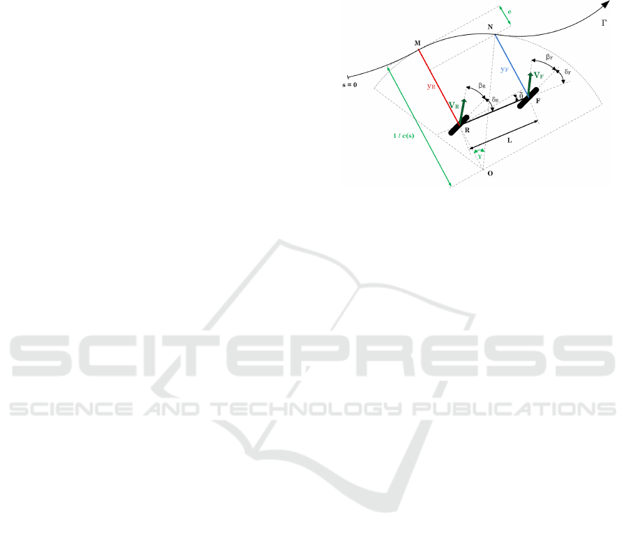
This point of view is depicted in Fig. 1.

Figure 1: Extended kinematic model of the robot with re-

spect to the reference trajectory Γ.

This robot of class {1,2}, according to the classi-

ﬁcation proposed by (Campion et al., 1996), is con-

trolled thanks to its rear velocity v

, dependent on the

wheel rotations, and the two steering angles : δ

for

the front axle, and δ

for the rear one. Classically, the

motion model is build under the rolling without slid-

ing assumption, imposing that the direction of each

speed vector is parallel to the tires. In off-road con-

texts, such an assumption is not valid, due to slip-

pages. As a result, the orientation of speed vectors

are different from the tire orientations (Canudas-de

Wit et al., 2001). An angle appears for each virtual

wheel (front and rear), which is named sideslip angle

and are denoted in this paper by β

for the front wheel

and β

for the rear one. These two angles are hardly

measurable directly and are assumed to be estimated

indirectly by the observer described in Sec. 3.

Assuming that sideslip angles are known, the front

and rear steering angles are considered to be the con-

trol variables of the system, since the velocity v

considered as a measured parameter, potentially vary-

ing. Thanks to this control variables, the objective of a

path tracking control law is to impose the convergence

of the robot w.r.t. the desired path Γ (see Fig. 1). The

tracking error y

is basically deﬁned as the minimal

distance between the middle of the rear axle R to Γ.

θ is the angular deviation, denoting the difference be-

tween the robot’s heading θ and the orientation of the

trajectory at the closest point of R belonging to Γ. At

this point, one can deﬁne the curvilinear abscissa s on

the path to be followed.

In this paper, we consider a second lateral devia-

tion with respect to the middle of the front axle (point

F). The distance between F and Γ is called the front

lateral deviation and is denoted by y

. In this paper,

ICINCO 2018 - 15th International Conference on Informatics in Control, Automation and Robotics

164

we consider that the wheelbase L (distance between F

and R) is small with respect to the curvature of the ref-

erence path at point M (denoted by c(s)). As a result,

the path to be followed may locally be approximated

by a circle whose radius is

c(s)

and whose centre is

O. In this paper, we consider a second lateral devia-

tion w.r.t. the middle of the front axle (point F), de-

noted y

. We consider that the intersection between

the straight line parallel to (MR) passing through the

point F, and the reference path Γ, is denoted N.

2.2 Global Motion Equations

As has been detailed in detailed in (Yi et al., 2009)

for the extended model depicted in Fig. 1, the motion

equation for the classical path tracking problem may

be expressed as:











s = v

cos(

)

1 − c(s)y

= v

sin(

θ = v

[cos(δ

+ β

)λ

− λ

(1)

with:











tan(δ

+ β

) − tan(δ

+ β

)

c(s) cos(

θ + δ

+ β

)

1 − c(s)y

θ + δ

+ β

(2)

This model is suitable for the path tracking ap-

proach since it can be turned into a linear form as

has been shown in (Morin and Samson, 2000), since

the extension to sideslip angles preserve the kinemat-

ical structure of mobile robots. As has been achieved

in (Lenain et al., 2010), this model permits to derive

a control law enabling the convergence of the rear lat-

eral deviation y

to zero. In particular, this is possible

whatever the value of the rear steering angle δ

, pro-

vided that its time derivative

can be neglected with

respect to the settling time of the control law imposed

on the front steering angle δ

. In the previous cited

reference, the rear steering angle is then used to con-

trol an angular deviation. If this permits to control

the heading of a robot independently from its lateral

position, it does not ensure explicitly the control of

the front axle position. As this paper aims at ensuring

the convergence of the position of the front and the

rear axle (point R and F) to the reference path Γ, an

additional model has to be introduced.

2.3 Modeling of the Two Subsystems

In order to ensure that both points of the robot chassis

F and R follow the same trajectory Γ, two models for

the derivative of tracking errors y

and y

are devel-

oped from the representation depicted in Fig. 1. The

dynamic of the rear lateral deviation y

is obtained

directly from the classical set of equation (2), i.e:

= v

sin(

(3)

Regarding the front axle, let us consider the geo-

metric properties in order to derive an expression of

with respect to y

. From Fig. 1, one can deﬁne the

relation (4),

= y

+ L sin(

θ) + e .

(4)

In this equation, only the deviation e remains un-

known. Assuming that, at each step, the trajectory is

locally (at any curvilinear abscissa s) viewed as a cir-

cle of radius

c(s)

, e can be expressed as:

e =

1 − cos(γ)

c(s)

(5)

where γ, depicted in Fig. 1 is the angle deﬁned by the

points [M O N]. This angle may be easily obtained

using the radius of curvature of the reference trajec-

tory, the angular deviation

θ and the robot wheelbase

γ = arcsin(Lc(s) cos(

θ)).

(6)

Thanks to this relation, the distance e is entirely

known and the lateral front deviation may be com-

puted thanks to the relation (2). The time derivative

may then be obtained, considering that e is slowly

varying with respect to the possible variation of y

thanks to actuator reactivity. It comes:

+ L

θ cos(

θ).

(7)

Using the global model, one can deﬁne an explicit

expression for the evolution of front lateral deviation:

= v

sin(

) + Lv

cos(

θ)[cos(δ

+ β

)λ

− λ

] .

(8)

The deﬁnition of λ

and λ

given in the model (2)

are explicitly linked to the control variable δ

and δ

Thanks to equations (3) and (2.3), the relationships

between the control variables and the time derivatives

of the lateral deviations are available. This constitutes

the model which will be used in Sec. 4 to derive the

control laws, provided that the sideslip angles β

and

are known, which is the aim of the observer de-

scribed hereafter.

Path Tracking of a Bi-steerable Mobile Robot: An Adaptive Off-road Multi-control Law Strategy

165

3 OBSERVATION OF SIDESLIP

ANGLES

In order to derive control laws for the convergence of

the lateral errors to zero, the knowledge of sideslip

angles is mandatory. There is no perception systems

allowing to measure directly such variables. Never-

theless, we assume that sensors on-boarded on the

robot permit to measure the position, the orientation

and the velocity of the robot at a given point, here

R. As it has been shown in (Lenain et al., 2014) and

extended to higher dynamic phenomena in (Deremetz

et al., 2017b), an observer may be built in order to es-

timate the two sideslip angles thanks to such a percep-

tion system. The details of the computation are in the

previous references. In this paper, the same approach

is used and only a short presentation is hereafter pro-

posed.

3.1 Observer State

In order to achieve the indirect estimation of sideslip

angles, let us consider the state space model ξ com-

posed of the robot lateral position and relative orien-

tation. Its evolution may be written as (9), based on

the model (2).

ξ =



dev





f (ξ

dev

, ξ

, v

, δ

)

2×1



(9)

where ξ is split into two sub-states:

• ξ

dev

= [y

θ]

, which constitutes the deviations of

the robot with respect to the trajectory Γ,

• ξ

= [β

]

, which is composed of the sideslip

angles, to be estimated.

The function f (ξ

dev

, ξ

, v

, δ

) is constituted

of the two last lines of the system (2). Because no

equation is available for the evolution of

and

in a kinematic representation, it is set to 0

2×1

. If the

observer gains are chosen appropriately, this model-

ing assumption is admissible, as it has been shown

in (Lenain et al., 2014). The objective of the observer

is to ensure the convergence of the complete observed

state

ξ to the actual ξ, measuring only the sub-state

dev

. As a result only the observation error related to

the deviation

dev

− ξ

dev

is known.

3.2 Observer Equations

It has been shown in (Lenain et al., 2014) that the

observer deﬁned by equation (10) permits the conver-

gence of the whole observed state

ξ to the actual one

ξ.







dev

= f (ξ

dev

, v

, δ

) + α

dev

(

dev

= α

(

dev

(10)

where α

dev

and α

are two functions of the obser-

vation error attached to the deviation part of the state

ξ, and deﬁned as follows:

(

dev

(

dev

) = K

dev

(

dev

) = K

∂ f

∂ξ

(ξ

dev

, v

, δ

)

dev

(11)

with K

dev

a 2 × 2 positive diagonal matrix and K

a positive scalar. These gains permit to tune the set-

tling time of the observer. As it can be seen consider-

ing (11), only the measurable error

dev

is mandatory

to compute the proposed observer. Thanks to this ap-

proach, the global model (2) may be entirely known.

As a consequence, expressions of front and rear lat-

eral deviation derivative (3) and (2.3) can be used to

compute control laws for the path tracking of points F

and R.

4 CONTROL LAWS

Thanks to the modeling proposed previously and the

observer deﬁned in (Lenain et al., 2014) and brieﬂy

presented in the previous section, a model linking lat-

eral deviations (front y

and rear y

) to the control

variables (steering angles and velocity) is available.

As a consequence, control laws on steering angles,

considering the velocity v

as a measured parameter

are here developed. This is achieved considering two

subsystems controlled by each steering angle.

4.1 Rear Steering Angle

Let us ﬁrst consider the regulation of the rear con-

trol point R on the trajectory. The objective is to en-

sure the convergence of the rear lateral deviation y

zero. The evolution of y

is related to the rear steer-

ing angle by the model (3), thanks to the intermediate

variable

. The convergence y

→ 0 may be ensured

by imposing the following differential equation:

= −K

(12)

with K

a positive scalar deﬁning the settling time for

the exponential convergence of y

to zero imposed

by (12). By injecting in this condition the expression

ICINCO 2018 - 15th International Conference on Informatics in Control, Automation and Robotics

166

of rear lateral error derivative (3), and using the deﬁ-

nition of

, one can reformulate the previous condi-

tions as:

= arcsin



−K



−

θ −

, (13)

provided that v

6= 0 and |

−K

|< 1. In practice,

in path tracking the velocity is always positive and

consequently non null, since the robot cannot be con-

trolled to its desired trajectory if it is stopped. Never-

theless, in order to permit stopping points to the robot,

one can deﬁne the gain K

as a function of velocity,

which has to be null when v

= 0. The second con-

ditions is linked to the existence range of the func-

tion arcsin. This impose that lateral error is small

enough with respect to the robot velocity and the gain:

| y

| v

. In practice, according to the values usu-

ally reached by velocity and the choice for the control

gain, the lateral deviation has to exceed several meters

in order to come across a singularity. When properly

initialized, such a value may hardly be reached. Nev-

ertheless, a saturation on error, or a variable gain may

be computed in order to avoid such a singularity.

The expression (13) constitutes the control law on

the rear steering angle in order to ensure the differen-

tial equation (12) on lateral deviation y

, implying its

convergence to zero.

4.2 Front Steering Angle

Once the rear steering angle is computed thanks to

the control law (13), the objective is to derive a con-

trol law for front steering in order to ensures the con-

vergence of the front steering (denoted by the point

F in Fig. 1) axle to the desired trajectory Γ. In other

words, the objective is to ensure the convergence of

the front lateral deviation to zero y

→ 0. Thanks to

the extended kinematic model computation, the ex-

pression (2.3) is available for the time derivative of

, pending on sideslip angles and steering angles.

One possible condition on

in order to permit the

convergence of y

to zero may be deﬁned as follows.

= −K

(14)

provided that K

is a positive scalar, the condi-

tion (14) will lead the front lateral error to exponen-

tially converge to zero. As rear steering angle δ

known, as well as sideslip angles (

and

are in-

deed on-line estimated thanks to the observer (10)),

one can introduce the explicit expression (2.3) for

in the previous condition. Computation permits to ex-

tract the following expression for front steering angle.

= arctan

(

Lλ

cos(δ

)

−

cos(δ

)cos(

θ)

− B

)

−

(15)

with B

sin(

)

cos(δ

)cos

− tan(δ

and λ

that are already deﬁned by the model (2), re-

placing sideslip angles by their corresponding obser-

vation values (i.e.

{F,R}

instead of β

{F,R}

). This con-

trol law for front steering angle exists under the same

conditions than those deﬁned for rear steering control

law. It has been designed using front and rear kine-

matic models deﬁned in Sec. 2, under the assumption

that the derivative of the rear sideslip angle and the

derivative of the rear steering angle are deﬁned as :

(

) = (0, 0). Such an assumption is considered

to be reasonable since the tuning of gain K

and K

can be achieved on this way (i.e. K

> K

). This

setting permits to emphasize reactivity of front axle

with respect to the rear one in order to meet such an

assumption. As pointed out in experimental results,

it does not affect the performances of the proposed

algorithm.

5 EXPERIMENTAL RESULTS

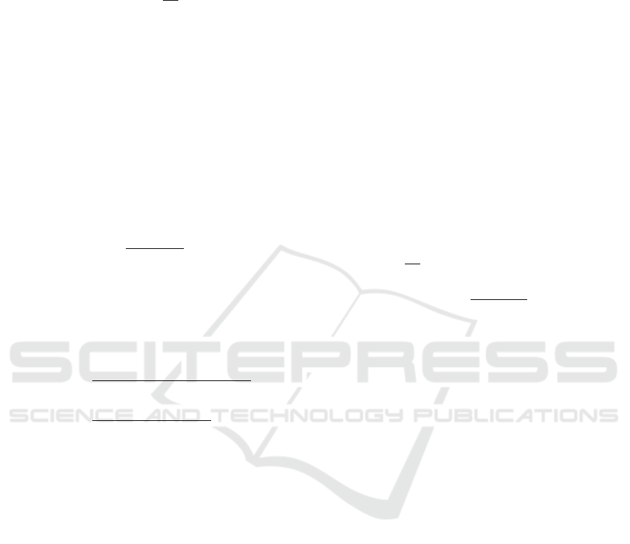
5.1 Experimental Setup

The four wheel-driven robot depicted in Fig. 2 is

used in order to point out the result of the pro-

posed approach. It is a fully electric mobile robot

equipped with four independent motors controlling

wheels speed. Two additionnal motors regulate the

front and rear steering angles. As shown in Fig. 2,

the main on-boarded sensor is an RTK-GPS settled

on the vertical of the rear axle (above the point R de-

picted in Fig. 1). It supplies the position within an

accuracy of ±2cm, while the heading is computed

thanks to a Kalman ﬁlter, mixing the GPS heading

data and the robot odometry. Related to the deﬁnition

of a reference path, these data permits to feed both

the observer, and the control laws (13) and (4.2). In

order to show the efﬁciency of the proposed control

algorithm, the autonomous tracking of the path de-

picted in Fig. 3 is ﬁrst realize by the robot using only

the front steering angle axle. The control in this case

is the approach proposed in previous works (Lenain

et al., 2014), based on the same observer, and using

predictive features.

Path Tracking of a Bi-steerable Mobile Robot: An Adaptive Off-road Multi-control Law Strategy

167

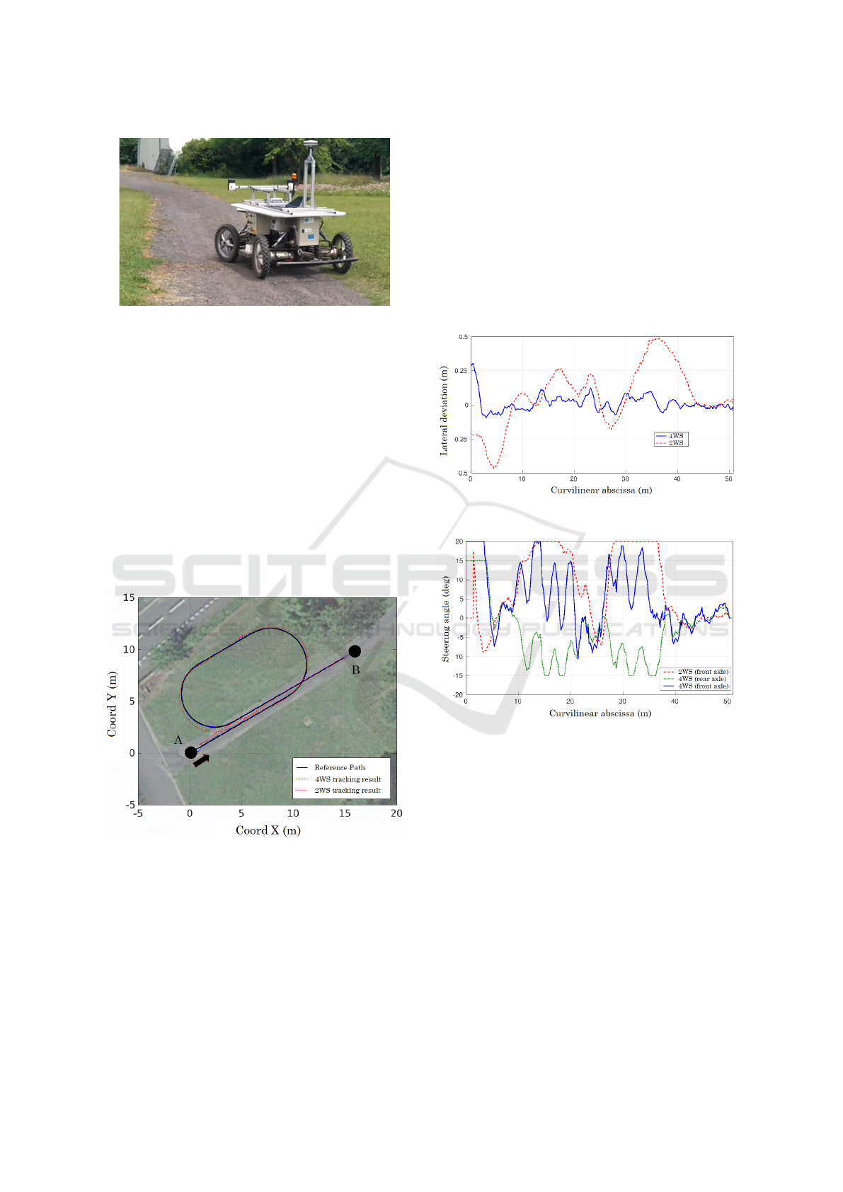
Figure 2: Experimental robot and on-boarded sensor.

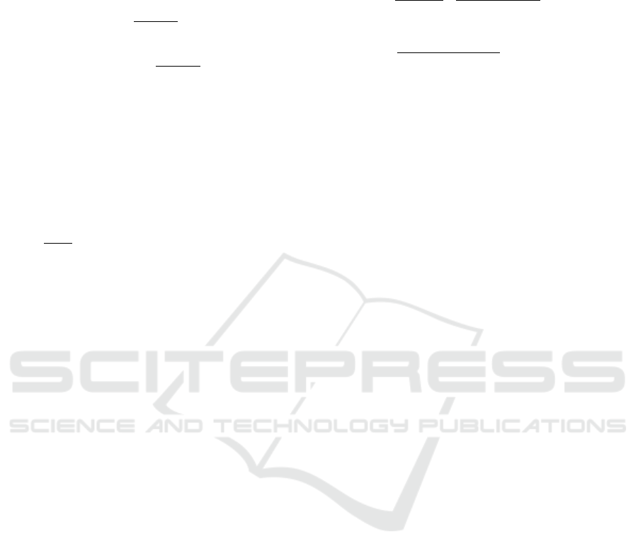
In order to highlight the beneﬁt of the proposed

four-wheel-steering control strategy, the reference tra-

jectory, depicted in black line in Fig. 3, has been pre-

viously recorded. This path, starting in A and ending

in B, is composed of straight line parts at the begin-

ning and the end, separated by two successive curves

with a radius of curvature equal to 3.4m and 3m re-

spectively. Such radii cannot be reached in practice

when controlling only the front steering wheels (lim-

ited to an angle of 20

◦

). As a result, the front steering

angle saturates and the robot cannot follow the trajec-

tory properly. This is pointed out by considering the

result of the path tracking depicted in red in Fig. 3,

achieved at 2m.s

−1

, with only the front steering acti-

vated.

Figure 3: Path to be followed and actually achieved trajec-

tories.

On the contrary, when using the front and rear

steering control strategy proposed in that paper, the

robot is able to track accurately the trajectory. The

successive positions recorded at 2m.s

−1

, when using

control laws (13) and (4.2) are indeed reported in blue

in Fig. 3, which are superimposed with the desired

trajectory.

5.2 Manoeuvrability Improvement in

Tracking Accuracy

The tracking accuracy obtained with and without us-

ing the control of the rear steering angle may be in-

vestigated in Fig. 4. The red dashed line depicts

the tracking error obtained when controlling only the

front steering axle. The large error obtained during

the curves (between curvilinear abscissa 15-25m and

30-42m) are due to the saturation of the front steering

axle, as reported in Fig. 5.

Figure 4: Comparison of tracking errors with and without

the use of rear steering angle.

Figure 5: Comparison of front steering angles, and rear

steering angle when used.

In this ﬁgure, the front steering angle obtained

when controlling the robot only with front steering

wheels is reported in dashed red line. It can be noticed

that the saturation value of 20

◦

is obtained almost all

the two bends. On the contrary, when using the front

and rear steering wheels, the front steering angle (de-

picted in blue plain line) is decreased thanks to the

rear steering angle (turning to the right), depicted in

green dotted line.

This permits to the robot to stay on the trajectory,

since the lateral deviation obtained when using the

proposed control strategy stay around zero, whatever

the curvature of the desired trajectory and the type

of ground (alternatively gravel and wet grass). This

tracking error is indeed depicted in blue plain line in

Fig. 4 and stays within ±10cm.

ICINCO 2018 - 15th International Conference on Informatics in Control, Automation and Robotics

168

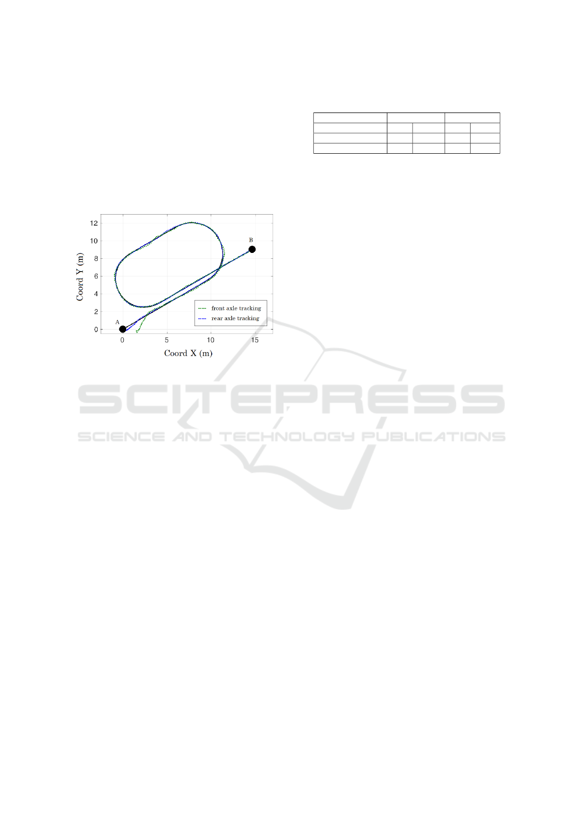
5.3 Trajectory of Each Axle

The second beneﬁt of this approach lies in the reduc-

tion of the space occupied by the robot during ma-

noeuvers, since front and rear axle follow the same

trajectory during the bend. This can be veriﬁed in

Fig. 6, where the trajectory of the front axle (point F)

is depicted in green dotted line (in addition to the ref-

erence trajectory depicted in black and the position of

point R depicted in blue).

Figure 6: Path to be followed and actually achieved trajec-

tories.

One can see that each point of the robot (R and

F) follows accurately the trajectory instead of hav-

ing a deviation in the front axle when using a single

steering axle robot. This permits to reduce the nec-

essary space to achieve harsh manoeuvres by increas-

ing the turning capabilities. As it can be seen on the

videos attached to the paper, using such an algorithm,

the robot is able to reach the trajectory without hav-

ing an angular deviation. During initialization phases,

the front and rear steering angles indeed rotate in the

same direction to cancel the initial lateral deviation.

In order to point out the accuracy obtained dur-

ing the tracking the Tab. 1 shows the statistical data

related to the absolute values of lateral deviations ob-

tained during the tracking. The mean and standard

deviation of the absolute value of the error recorder

at points R (y

) and F (y

) are reported for the track-

ing results using the proposed approach and compared

to the data obtained using the front steering angle.

It can be noticed that when using the proposed ap-

proach, the mean and standard deviations are very

close to zero (a few centimetres accuracy), despite of

the harsh radius of curvature imposed by the path to

be followed. On the contrary, when using a single

steering axle (front), since saturations occurred, large

deviations may be recorded leading to a bad accuracy

(with a mean of more than 30cm, for the front steer-

ing point). This value is logicallly bigger than for the

rear control point R (22cm) since only the position of

Table 1: Comparison of absolute value of lateral deviation

recorded during the tracking.

2 steering angles 1 steering angle

| y

| | y

mean (m) 0.04 0.07 0.22 0.32

standard deviation (m) 0.03 0.05 0.19 0.27

point R is controlled when a single steering angle is

controlled.

When using the proposed control laws (13)

and (4.2), it can be noticed than the front lateral devi-

ation y

is a little bit less accurate than the rear one y

(7cm against 4cm). This is due to the small deviations

of the point F which can be noticed in Fig. 6. This

can be explained by the fact that the control law for

the front steering angle (4.2) does not account for the

variations of rear steering angle δ

. When fast vari-

ations of δ

occurs, a settling time is mandatory for

the front axle to compensate for these variations. As

a results, some punvtual overshoots can be recorder.

This may be tackled in future works by using predic-

tive control.

6 CONCLUSIONS

In this paper a new control algorithm dedicated to four

wheel-driven mobile robot is proposed. The front and

rear axle of the robot are considered as two indepen-

dent sub-systems regulating their own point on the

same desired trajectory. The physical link is ensured

by the computation of the front tracking error, which

is deduced from the rear position and the robot’s head-

ing. An adaptive approach is added from previous

work in order to face the potential inﬂuence of bad

grip conditions, since such works are devoted to off-

road application, such as in civil security or in agricul-

ture, for which high manoeuvrability is mandatory.

Experimental results have shown the efﬁciency of the

proposed approach at low speed (up to 2m.s

−1

), for

which the dynamical effects can be neglected. Fu-

ture works are focused on the increase of the robot

speed. A predictive layer, exploiting the knowledge

of the path to be followed is expected to be imple-

mented to compensate for inertial effects and the in-

ﬂuence of low level delays. Moreover, control laws

proposed explicitly relies on the velocity and do not

exist when the robot stops. This impose to switch the

control laws to zero when the velocity is close to zero.

To overcome this drawback, a new version will be

proposed, based on a model using partial derivative

of error with respect to curvilinear abscissa, instead

of time derivatives.

Path Tracking of a Bi-steerable Mobile Robot: An Adaptive Off-road Multi-control Law Strategy

169

ACKNOWLEDGEMENTS

This work has been sponsored by the French govern-

ment research program ”Investissements d’Avenir”

through the IMobS3 Laboratory of Excellence (ANR-

10-LABX-16-01), by the European Union through

the program ”Regional competitiveness and employ-

ment 2007-2013” (ERDF Auvergne region), and by

the Auvergne region.

It received the support of French National Research

Agency under the grant number ANR-14-CE27-0004

attributed to Adap2E project (adap2e.irstea.fr) and

has also been sponsored through the RobotEx Equip-

ment of Excellence (ANR-10-EQPX-44). We thank

them for their ﬁnancial support.

REFERENCES

Ackermann, J. (1994). Robust decoupling, ideal steering

dynamics and yaw stabilization of 4ws cars. Automat-

ica, 30(11):1761–1768.

Anderson, R. and Bevly, D. (2005). Estimation of tire cor-

nering stiffness using GPS to improve model based es-

timation of vehicle states. In IEEE Intelligent Vehicles

Conference, Las Vegas, U.S.A.

Blackmore, C. (2014). Learning to change farming and

water management practices in response to the chal-

lenges of climate change and sustainability. Outlook

on AGRICULTURE, 43(3):173–178.

Campion, G., Bastin, G., and Andr

ea-Novel, B. d. (1996).

Structural properties and classiﬁcation of kinematic

and dynamic models of wheeled mobile robots. IEEE

Transactions on Robotics and Automation, 12(1):47–

62.

Canudas-de Wit, C., Tsiotras, P., Claeys, X., Yi, J., and

Horowitz, R. (2001). Friction tire/road modeling, esti-

mation and optimal braking control. In NACO2 Work-

shop, Lund, Sweden, volume 45.

Cariou, C., Lenain, R., Thuilot, B., and Berducat, M.

(2009). Automatic guidance of a four-wheel-steering

mobile robot for accurate ﬁeld operations. Journal of

Field Robotics, 26(6-7):504–518.

Deremetz, M., Lenain, R., Couvent, A., Cariou, C., and

Thuilot, B. (2017a). Path tracking of a four-wheel

steering mobile robot: A robust off-road parallel steer-

ing strategy. In Mobile Robots (ECMR), 2017 Euro-

pean Conference on, pages 1–7. IEEE.

Deremetz, M., Lenain, R., Thuilot, B., and Rousseau, V.

(2017b). Adaptive trajectory control of off-road mo-

bile robots: A multi-model observer approach. In

Robotics and Automation (ICRA), 2017 IEEE Inter-

national Conference on, pages 4407–4413. IEEE.

Grimstad, L., Pham, C. D., Phan, H. T., and From, P. J.

(2015). On the design of a low-cost, light-weight,

and highly versatile agricultural robot. In Advanced

Robotics and its Social Impacts (ARSO), 2015 IEEE

International Workshop on, pages 1–6. IEEE.

Haibo, L., Shuliang, D., Zunmin, L., and Chuijie, Y. (2015).

Study and experiment on a wheat precision seeding

robot. Journal of Robotics, 2015:12.

Lefvre, S., Carvalho, A., and Borrelli, F. (2015). Au-

tonomous Car Following: A Learning-Based Ap-

proach. IEEE Intelligent Vehicles \ldots.

Lenain, R., Thuilot, B., Cariou, C., and Martinet, P. (2010).

Mixed kinematic and dynamic sideslip angle observer

for accurate control of fast off-road mobile robots.

Journal of Field Robotics, 27(2):181–196.

Lenain, R., Thuilot, B., Guillet, A., and Benet, B. (2014).

Accurate target tracking control for a mobile robot: a

robust adaptive approach for off-road motion. In IEEE

International Conference on Robotics and Automation

(ICRA).

Morin, P. and Samson, C. (2000). Practical stabilization

of a class of nonlinear systems. Application to chain

systems and mobile robots. In IEEE Conference on

Decision and Control (CDC), volume 3, pages 2989–

2994, Sydney (Australia).

Nizard, A., Thuilot, B., Lenain, R., and Mezouar, Y. (2016).

Nonlinear path tracking controller for bi-steerable ve-

hicles in cluttered environments. IFAC-PapersOnLine,

49(15):19–24.

Peng, S.-T. P. S.-T., Sheu, J.-J. S. J.-J., and Chang, C.-C.

C. C.-C. (2004). A control scheme for automatic path

tracking of vehicles subject to wheel slip constraint.

In Proceedings of the 2004 American Control Confer-

ence, volume 1, pages 804–809 vol.1.

Raksincharoensak, P., Nagai, M., and Mouri, H. (2001).

Investigation of automatic path tracking control us-

ing four-wheel steering vehicle. In IVEC2001. Pro-

ceedings of the IEEE International Vehicle Electron-

ics Conference 2001. IVEC 2001 (Cat. No.01EX522),

pages 73–77.

Wang, D. and Qi, F. (2001). Trajectory planning for a four-

wheel-steering vehicle. In Robotics and Automation,

2001. Proceedings 2001 ICRA. IEEE International

Conference on, volume 4, pages 3320–3325. IEEE.

Yi, J., Wang, H., Zhang, J., Song, D., Jayasuriya, S., and

Liu, J. (2009). Kinematic modeling and analysis of

skid-steered mobile robots with applications to low-

cost inertial-measurement-unit-based motion estima-

tion. IEEE Transactions on Robotics, 25(5):1087–

1097.

ICINCO 2018 - 15th International Conference on Informatics in Control, Automation and Robotics

170