Nonlinear Design of Model Predictive Control

Adapted for Industrial Articulated Robots

etoslav Belda

Department of Adaptive Systems,

The Czech Academy of Sciences, Institute of Information Theory and Automation,

Pod Vod

arenskou v

ı 4, 182 08 Prague 8, Czech Republic

Keywords:

Discrete Model Predictive Control, Nonlinear Design, Lagrange Equations, Articulated Robots.

Abstract:

This paper introduces a speciﬁc nonlinear design of the discrete model predictive control based on the features

of linear methods used for the numerical solution of ordinary differential equations. The design is intended

for motion control of robotic or mechatronic systems that are usually described by nonlinear differential equa-

tions up to the second order. For the control design, the explicit linear multi-step methods are considered.

The proposed way enables the design to apply nonlinear model to the construction of equations of predictions

used in predictive control. An example of behavior of proposed versus linear predictive control is demonstrated

by a comparative simulation with nonlinear mathematical model of six-axis articulated robot.

1 INTRODUCTION

The number of industrial robots increases steadily.

Such trend proceeds with the advent of Industry 4.0

also in the immediate future (Colombo et al., 2016).

The robots in industrial production perform thou-

sands of operations. Their efﬁciency depends highly

on the adequate motion control that can employ avai-

lable pieces of information from user and real data

(Chung et al., 2016).

Nowadays, necessary information, data and com-

puting power are broadly available, however, the de-

signers have to combine them effectively. In indus-

trial production, there exist a lot of elaborated strate-

gies that follow from long-term, empirical experien-

ces (SPS IPC Drives, 2017). Unfortunately, such stra-

tegies are usually not universal enough. They are not

scalable or simply transferable for general use in dif-

ferent or modiﬁed systems.

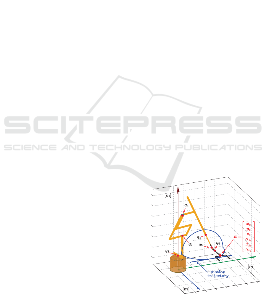
From mathematical point of view, the robots, ma-

nipulators, such as a mechanical structure of articu-

lated robot class depicted in Fig. 1, represent dyn-

amic systems that are usually described by systems

of ordinary differential equations (ODEs) forming

appropriate dynamic models (Siciliano et al., 2009).

Such models can be considered as a proper substitu-

tion of the real physical robot mechanism for com-

puter simulations and motion control design as well.

The mentioned systems of ODEs, include vari-

ous relations among individual elements of the ro-

bot constructions. These relations tend to be non-

linear due to the presence of nonlinear operations

on descriptive variables and their appropriate deri-

vatives such as multiplication, division, goniometric

functions etc. (Arimoto, 1996). Thus, conventional

linear control theory (Wang, 2009) cannot be directly

exploited without modiﬁcations.

axis y

0.1

0.2

0.3

-0.2

0.4

0.5

0.6

0.5

0.2

0.4

0.3

0.2

0.1

axis

axis x

Figure 1: Wire-frame model of the articulated robot class.

Belda, K.

Nonlinear Design of Model Predictive Control Adapted for Industrial Articulated Robots.

DOI: 10.5220/0006833500710080

In Proceedings of the 15th International Conference on Informatics in Control, Automation and Robotics (ICINCO 2018) - Volume 2, pages 71-80

ISBN: 978-989-758-321-6

In engineering practice, there exist several usual

solutions. They are based on local linearization (Os-

tafew et al., 2016) by means of Taylor series, par-

tial derivative models or switching local linear models

with an inclusion of discretization to obtain discrete

linear-like model, often in state-space form. Then,

usual linear design of discrete model predictive con-

trol can be applied (Ordis and Clarke, 1993; Macie-

jowski, 2002; Wang, 2009; Belda et al., 2007; Belda

and Vo

smik, 2016; Belda and Rovn

y, 2017). Succee-

ding approaches use linear models with stochastic un-

certainties substituting locally initial nonlinear model

(Kothare et al., 1996). Other solutions can be realized

by neural network (Negri et al., 2017) or by the di-

rect nonlinear optimization such as in (Kirches, 2011;

Houska et al., 2011; Wilson et al., 2016; Faulwasser

et al., 2017; Zanelli et al., 2017). However, they do

not represent immediately applicable, straightforward

multi-step design in each time-instant of the control

process.

This paper introduces a novel way of the design

of the discrete model predictive control that howe-

ver employs a continuous-time nonlinear ODE model

of the robot dynamics. The model is employed di-

rectly by means of speciﬁcally adapted explicit linear

multi-step numerical methods without any lineariza-

ton and conventional model discretization. The nume-

rical methods are used for the construction of equati-

ons of predictions. These equations can be involved

in usual way to the regular quadratic cost function

and optimization criterion. The explanation is intro-

duced with Adams-Bashforth method as a representa-

tive of the aforementioned explicit methods (Butcher,

2016). A summary of the features of the proposed so-

lution is involved including its comparison with usual

linear design of model predictive control (Ordis and

Clarke, 1993; Wang, 2009) considering conventio-

nal repeated linearization and discretization in com-

pliance with the robot motion.

2 NONLINEAR ROBOT MODEL

The model of the considered class “articulated robots”

is generally represented by a nonlinear function des-

cribing relations between control actions (robot in-

puts, joint torques τ = τ (t)) and descriptive varia-

bles (robot outputs, joint angles and their derivatives

q = q(t), ˙q = ˙q(t) and ¨q = ¨q(t)):

¨q = f(q, ˙q, τ) (1)

The model (1) represents equations of motions (Sici-

liano et al., 2009; Othman et al., 2015) that describe

robot dynamics.

Such a model is mostly composed by Lagrange

equations, e.g. in the following form



∂E

∂ ˙q



−



∂E

∂q





∂E

∂q



= τ (2)

where q, ˙q, E

, E

and τ are generalized coordina-

tes and their appropriate derivatives, total kinetic and

potential energy and vector of generalized force ef-

fects associated with generalized coordinates (Sicili-

ano et al., 2009).

The individual terms in the equation system (2)

can be deﬁned as follows



∂E

∂ ˙q



H(q, ˙q) ˙q + H(q) ¨q (3)

−



∂E

∂q



= S(q, ˙q) ˙q −

H(q, ˙q) ˙q (4)



∂E

∂q



= g(q) (5)

where, considering simpliﬁed notation, the matrices

H =H(q), S = S(q, ˙q) and

H =

H(q, ˙q) =

(H(q))

relate to inertia effects and vector g = g(q) corre-

sponds to effects of gravity. Thereafter, the model

(equations of motion of articulated robots) can be de-

ﬁned as follows

¨q =

f(q, ˙q, τ )

z }| {

−H

−1



H + S



˙q

| {z }

f(q, ˙q)

− H

−1

| {z }

(q)

| {z }

(q, ˙q)

+ H

−1

| {z }

(q) τ

= f (q, ˙q) + u (6)

where the terms f (q, ˙q) = −H

−1



H + S



˙q

and u = H

−1

(−g + τ).

Thus, equation (6) can be introduced as a particu-

lar expression of the model (1) as follows

¨q = f

(q, ˙q) + g

(q) τ = f (q, ˙q) + f

(q) + g

(q) τ

= f (q, ˙q) + g(q) u (7)

where g(q) is added just for the generality; it is iden-

tity matrix here. In (7), the effects of gravity f

(q) are

incorporated into robot inputs as outer forces consi-

dering their static and ﬁxed character that cannot be

reduced or suppressed in the control design.

Note that ﬁnal torques required on drives (refe-

rence torques for drive control) are given by

τ = H u + g (8)

ICINCO 2018 - 15th International Conference on Informatics in Control, Automation and Robotics

3 INTEGRATION CONCEPT

To obtain discrete form of nonlinear predictive cont-

rol, let us consider individual time instants of the ini-

tial continuous nonlinear function in the model (1)

as follows (i.e. sampling, no model discretization)

= f(q, ˙q, τ )|

t = k T

, k = 0, 1, ··· (9)

where T

is suitably selected sampling period. Let us

apply the same to the terms from (7)

= f (q, ˙q) g

= g(q) |

t = k T

(10)

The statements (9) or (10) will be suitable for a speci-

ﬁc construction of the predictions relative to unknown

control actions u(t) within ﬁnite discrete time set

t ∈ {k T

, (k+1) T

, ··· , (k+N −1) T

}, where N

is a prediction horizon.

The predictions still take into account the continu-

ous nonlinear model, but only in the indicated discrete

time samples for discrete design of predictive control.

Such a concept can be realised by means of numeri-

cal methods (Butcher, 2016) used for the numerical

approximation of the solution of the ﬁrst-order ordi-

nary differential equations (ODEs):

˙y = f(t, y) with initial condition y

= y|

t = 0

(11)

Speciﬁcally, these methods are used to ﬁnd a numeri-

cal approximation of the exact integral over a speciﬁc

time interval, e.g. t ∈ hk T

, (k+1) T

k+1

= y

(k+1) T

k T

˙y dt = y

(k+1) T

k T

f(t, y) dt

ˆy

k+1

= y

+ h δ(t, y) (12)

where y

= y|

t=k T

is an initial condition of the con-

sidered time interval, ˆy

k+1

is an approximation

of the exact solution y

k+1

= y|

t=(k+1) T

, δ(t, y) re-

presents generally the function approximating ˙y so

that ˆy

k+1

would be the adequate approximation of

k+1

and h is a step of integration method, which is

selected as h = T

From wide range of the methods, let us focus on

linear multi-step methods suitable for the predictions

in predictive design. Generally, linear multi-step met-

hods are deﬁned as

ˆy

k+1

i=0

k−i

+ h

j=−1

k−j

(13)

where ˆy

k+1

is a result of the numerical integration

based on the previous y

k−i

For the design, the explicit methods are useful

such as explicit Adams-Bashforth method of fourth

order with r = 0, α

= 1, s = 3 and β

j ∈ {−1, 0, 1, 2, 3}, where γ

−1

= 0, γ

= 55,

= −59, γ

= 37 and γ

= −9, as follows

ˆy

k+1

= y

+ h ( −

k−3

k−2

−

k−1

) (14)

Thus, for completeness, the function approximating ˙y

from (12) is as follows:

δ(t, y) = −

k−3

k−2

−

k−1

The aforementioned Adams-Bashforth linear method

(Butcher, 2016) will be used in the next explanation

of the following section.

4 NONLINEAR DESIGN

OF PREDICTIVE CONTROL

The nonlinear model predictive design focusses re-

cently on the solution of nonlinear optimal control

problem with integral criterion of optimality. It repre-

sents general solution using sophisticated nonlinear

optimization algorithms. But it leads to sequential

quadratic programming (QP) representing one-ahead

spreading-in-time-optimization process, thus iterati-

vely approximating the nonlinear problem with QP

(Faulwasser et al., 2017; Zanelli et al., 2017). Al-

ternatively, the usual summation form of the criterion

used in linear control theory can be also taken into ac-

count. The operation of integration is just shifted

from the criterion towards predictions via continuous-

time model represented by ODEs. This idea will be

used and introduced in the proposed design.

Let us start from the continuous model (7) con-

sidered in the discrete time samples (time instants)

as was designated in (10). Moreover, let us use more

common, universal notation for outputs y instead of q,

i.e. y

= q

as well as for appropriate derivatives

˙y

= ˙q

and ¨y

= ¨q

¨y

= f

+ g

(15)

From (6), the function f

holds f

[ ˙y = 0, y ∈R)]

= 0

whereas term f

g k

y ∈ R

6= 0 in (7) for the conside-

red spatial articulated robot class as well as for ver-

tical planar robot conﬁgurations. For completeness,

g k

y ∈ R

= 0 applies to horizontal planar robot con-

ﬁgurations. The property of f

is helpful for the sta-

bility of the control design.

Using the model (15), the speciﬁc design

of the nonlinear model predictive control can be now

explained within the following three sections.

Nonlinear Design of Model Predictive Control Adapted for Industrial Articulated Robots

4.1 Criterion and Cost Function

The criterion for predictive control design can gene-

rally be written as follows

min

(

k+1

, W

k+1

, U

)

(16)

subject to:

k+1

= f (y

, ˙y

, δ(t, y, ˙y))

¨y

= f

+ g

where δ(t, y, ˙y) follows from the second order model

¨y

= f

+ g

, where f

= f (y, ˙y) as in (10).

k+1

, W

k+1

and U

stand for the sequences

of the robot output predictions, references and cont-

rol actions, respectively

k+1

= [ˆy

k+1

, ··· , ˆy

k+N

]

(17)

k+1

= [w

k+1

, ··· , w

k+N

]

(18)

= [u

, ··· , u

k+N −1

]

(19)

Then the cost function J

is selected in common

quadratic form as follows

i=1

{||Q

(ˆy

k+i

− w

k+i

)||

+ ||Q

k+i−1

}

k+1

− W

k+1

)

Y W

(

k+1

− W

k+1

)

+ U

(20)

where Q

Y W

and Q

are penalizations

deﬁned as









∗

0 Q

∗







(21)

where the symbolic subscripts

, ∗ have the following

interpretation:  ∈ {Y W, U} and ∗ ∈ {yw, u}.

However, the function can be selected variously

according to user requirements, e.g. considering

incremental terms that can slightly moderate

and smooth the robot motion (Maciejowski, 2002)

or suppress steady-state control error (Wang, 2009;

Belda and Z

ada, 2017).

4.2 Equations of Predictions

As was already mentioned, the equations of predicti-

ons will be composed with the nonlinear continu-

ous model (15) and by means of the idea of the ap-

proximation of the exact integral as indicated in (12)

by the exemplarily selected linear multi-step Adams-

Bashforth method of fourth order (14) for the solution

of the ﬁrst-order ODEs.

However, the nonlinear model of the robot (15) re-

presents a system of the second-order ODEs. To ap-

ply the selected suitable numerical method, but wit-

hout lost of information about included nonlinear re-

lations, the model (15) has to be speciﬁcally rearran-

ged into ODEs of the ﬁrst order. For the necessary re-

arrangement, the following backward Euler formula

can be selected for simplicity

˙y

k+1

ˆy

k+1

− y

(22)

The used formula ensures coupling (propagation)

of nonlinear relations from (15) into positional esti-

mates, since the numerical methods represent only li-

near combinations within rows of the ODEs. Thus,

usual rearrangement via addition of further ODEs de-

creasing the order of initial ODE system would not be

helpful.

Taking the aforementioned features into account,

then the positional estimate ˆy

k+1

can be evaluated

by the velocity estimate

˙y

k+1

, which includes fully

the initial nonlinear model (15), as follows

ˆy

k+1

= y

+ h

˙y

k+1

(23)

where the estimate

˙y

k+1

is given generally by the nu-

merical integration of the ODE set as follows

˙y

k+1

= ˙y

+ h δ(t, y, ˙y) (24)

Note, for completeness, if the appropriate robot

model would be set of ﬁrst-order ODEs only, i.e.

˙y

+ ˜g

as e.g. in (Groothuis et al., 2017; Z

ada and Belda,

2017), this step is omitted.

Now, the pure equations of predictions can

be composed considering the model (15), a spe-

ciﬁc numerical method (24) (here, the Adams-

Bashworth (14) is selected) and the rearrangement

to the ﬁrst-order ODE set as indicated by (23).

ICINCO 2018 - 15th International Conference on Informatics in Control, Automation and Robotics

The equations of predictions in a matrix form are

deﬁned for the velocity vector

as follows

k+1

= ˙y

+ F

+ G

(25)

and as well as for the position vector

k+1

= y

+ L

+ M

(26)

where the individual terms represent multiple identity

matrix: F

= [ I ···I ]

, speciﬁc free responses:

“ ˙y

”, “ y

” and forced responses:

“ G

”, “ M

”, respectively.

and G

can be derived from the following sequen-

ces for velocities, where, for clarity, individual time

steps are separated by horizontal lines:

˙y

k+1

= ˙y

+ F

1,k

+ β

1,k

= β

¨y

k−3

+ β

¨y

k−2

+ β

¨y

k−1

+ β

˙y

k+2

= ˙y

+ F

2,k

+ (β

+ β

) g

+ β

ˆg

k+1

2,k

1,k

+β

¨y

k−2

+β

¨y

k−1

+β

k+1

˙y

k+N

= ˙y

N,k

+ {

j=0

+ ··· + β

ˆg

k+N −1

N,k

= F

N−1,k

j=1

j−1

k+N−j

(27)

Note that in step k, the topical value ˙y

as well as

its appropriate past values ˙y

k−1

, ˙y

k−2

and ˙y

k−3

are

known from measurements or some state estimation.

Consequently, vector F

from (25) can be deﬁned

in the following way:







1, k

2, k

N, k







(28)

Similarly, the matrix G

from (25) is deﬁned as







0 ··· 0

(β

+ β

) g

ˆg

k+1

{

j=0

··· ··· β

ˆg

k+N −1







(29)

where

k+i

and ˆg

k+i

can be substituted by fu-

ture reference values as

k+i

= f

k+i

, ˙w

k+i

)

and ˆg

k+i

= g

k+i

Similarly in the construction of the equations (26),

k+1

, L

and M

can be deﬁned by analogical se-

quences for positions as follows (again for clarity, in-

dividual time steps are separated by horizontal lines):

ˆy

k+1

= y

+ L

1, k

+ h β

1, k

= h ˙y

+ h F

1, k

ˆy

k+2

= y

+ L

2, k

+h (β

+ 2 β

) g

+h β

ˆg

k+1

2, k

= L

1, k

+ h F

2, k

ˆy

k+N

= y

+ L

N, k

+ h {

j=0

(N−j)β

+ ··· + hβ

ˆg

k+N −1

N, k

= L

N−1, k

+ h F

N, k

(30)

Then, vector L

and matrix M

from (26) are:







1, k

2, k

N, k







(31)







h β

0 ··· 0

h (β

+2 β

) g

h β

ˆg

k+1

j=0

(N−j)β

··· ··· h β

ˆg

k+N −1







(32)

Note that due to second order ODEs, the two-step

equations of predictions (25) and (26) are used here.

Nonlinear Design of Model Predictive Control Adapted for Industrial Articulated Robots

4.3 Square-root Minimization

To minimize cost function (20), let us consider the fol-

lowing expression

min

= min

⇒ min

(33)

indicating the square-root minimization of the vec-

tor J

instead of minimization of the scalar J

where the square-root minimization is more suitable

from computation point of view. Thus, the square-

root of the criterion (16) with the cost function (20)

is as follows

min

= min



Y W

0 Q



k+1

− W

k+1



(34)

which can be solved as a speciﬁc least-square pro-

blem by the following system of algebraic equations

(Lawson and Hanson, 1995) that involves equations

of predictions (26) for

k+1



Y W





Y W

k+1

−y

−L

)



(35)

The system (35), that is over-determined, can

be written in condensed general form (36). This

form can be transformed to another form (37)

by orthogonal-triangular decomposition (Lawson and

Hanson, 1995) and solved for unknown U

= b (36)

= Q

b assuming that A = Q R

= c

(37)

where Q

is an orthogonal matrix that transforms ma-

trix A into upper triangle R

as indicated

⇒

(38)

Vector c

represents a loss vector, Euclidean norm

||c

|| of which equals to the square-root of the op-

timal cost function minimum, scalar value

√

i.e. J = c

. Only the ﬁrst elements corresponding

to u

are selected from computed vector U

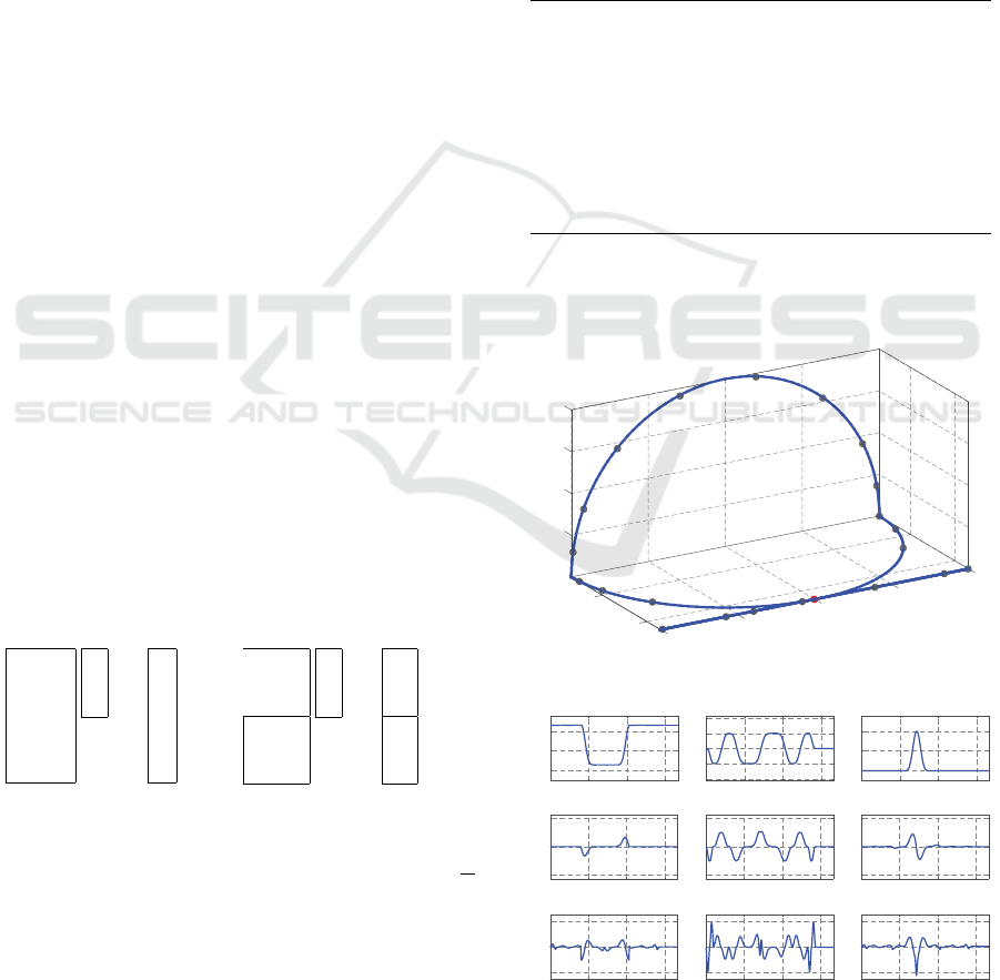
5 SIMULATION EXAMPLE

The example demonstrates the behavior of the articu-

lated robot along selected testing trajectory. The cor-

responding wire-frame model including trajectory

is shown in Fig. 1. Trajectory in detail is in Fig. 2

and Fig. 3.

The depicted trajectory in Fig. 1 was time para-

meterized with acceleration polynomial of ﬁfth-order

(Siciliano et al., 2009; Belda and Novotn

y, 2012).

The speciﬁcation of individual trajectory segments is

listed in the Table 1

Table 1: Testing trajectory in G code (mm).

001: N010 G19

002: N020 G00 X630 Y-200 Z400

003: N030 G00 X630 Y200 Z400

004: N040 G00 X630 Y0 Z400

005: N050 G02 X430 Y-200 Z400 I-200 J0 K0

006: N060 G02 X430 Y200 Z400 I0 J200 K0

007: N070 G02 X630 Y0 Z400 I0 J-200 K0

008: N080 G00 X630 Y-200 Z400

009: N090 G00 X630 Y200 Z400

010: N010 G00 X630 Y0 Z400

where G19, G00 and G02 are commands for plane se-

lection, linear and circular interpolation, respectively.





















































































Figure 2: Testing trajectory with speciﬁc time marks.



































































































































































Figure 3: Cartesian coordinates and derivatives (time in (s)).

ICINCO 2018 - 15th International Conference on Informatics in Control, Automation and Robotics



D[LV







D[LV







D[LV







D[LV





E =



D[LV







D[LV







D[LV







D[LV







D[LV







D[LV







D[LV







D[LV





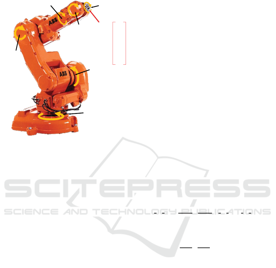
Figure 4: Six-axis multipurpose ABB robot IRB 140.

The used dynamic model (7) and (8) from (2)-(6)

had parameters of ABB robot IRB 140 (Fig. 4).

The number of actuated (driven) axes of the ro-

bot is six as well as a number of degrees of freedom

of the robot. Six degrees of freedom correspond to six

inputs: torques τ

1:6

(N·m), six outputs: joint coordi-

nates y = q

1:6

(rad) relating to the appropriate Car-

tesian coordinates:

E = [ {x

, y

, z

(m)}, {α

, β

, γ

(rad) }]

and twelve state variables:

x = [ q

1:6

(rad), ˙q

1:6

(rad ·s

−1

) ]

corresponding to joint coordinates and their appropri-

ate derivatives.

Note that end-effector was oriented to be parallel

with axis x

. Thus, the orientation angles are consi-

dered to be constant:

= β

= γ

= 0 rad

However, corresponding reference values in joint

space w

1:6,∀k

, k = 1, 2, ··· , are changing accor-

ding to appropriate kinematic transformation speciﬁc

for considered robot.

5.1 Simulation Setup

Proposed nonlinear design of model predictive cont-

rol (NdMPC) was tested with the following parame-

ters:

- sampling period: T s = 0.01s

- horizon of prediction: N = 10

- output penalization: Q

= I

(6×6)

- input penalization: Q

= 2 · 10

−4

(6×6)

where I is the identity matrix.

The proposed algorithm was compared with regular

model predictive control (MPC) (Wang, 2009) having

identical setting. The MPC, used for the comparison,

was as follows

= (

Y W

+ Q

)

−1

Y W

k+1

−

)

(39)

where matrices

F and

G are derived from the initial

nonlinear model (7) as follows



















··· 0

N−1

··· CB







(40)

Linear-like matrices A

and B

, involved in (40),

are obtained conventionally by model linearization

and discretization repeating in every time instant k.

C is an output matrix. All terms follow from state-

space form:



˙y

¨y



| {z }

˙x



0 I

0 f( ˙y, y)



| {z }

A(t)



˙y



| {z }





| {z }

u (41)

y =



I 0



| {z }



˙y



(42)

that is discretized: A(t), B |

⇒ A

, B

by ﬁrst-

order-hold method (Franklin et al., 1998) and arran-

ged as

k+1

= C A

+ C B

(43)

The details on used MPC can be found e.g. in (Ordis

and Clarke, 1993; Wang, 2009).

5.2 Summary of the Results

The simulation was performed with the mentioned

setting and with artiﬁcially added mismatch between

the model used for the control design and the mo-

del for simulation. The mismatch consisted in the

four-times increased weight of the last, 6

robot link

in the simulation model against model for the design,

i.e. m

= 0.25kg and ˜m

= 4×m

Nonlinear Design of Model Predictive Control Adapted for Industrial Articulated Robots

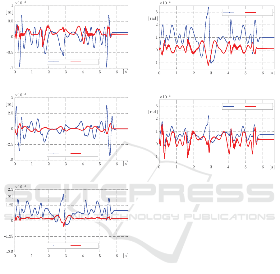
Å-0# Å.d-0#

Figure 5: Time histories of errors in the axis x.

Å-0#

Å.d-0#

Figure 6: Time histories of errors in the axis y.

Å-0# Å.d-0#

Figure 7: Time histories of errors in the axis z.

The Fig.5 - Fig.7 show control errors at the ro-

bot motion along the testing trajectory. They represent

the errors in Cartesian coordinate system. The values

of the appropriate Cartesian coordinates were recom-

puted from ‘measured’ values of joint coordinates.

The corresponding errors in the joint space

for the most exposed joints q

and q

to load are

shown in Fig. 8 and Fig. 9. The exposition is caused

by the robot motion itself, thus its character across

the symmetry plane x

= 0

. The mentioned

ﬁgures show the lower tracking errors for the pro-

posed method. Considering moving-mass distribu-

tion in the robot: m

= 35 kg, m

= 16 kg,

= 14 kg, m

= 6 kg, m

= 0.75kg

and m

= 0.25kg, then the highest vertical load

is on 2

link between joints q

and q

, which is ac-

-0#

Å.d-0#

Figure 8: Time histories of control error for joint q

-0#

Å.D-0#

Figure 9: Time histories of control error for joint q

tuated in joint q

For the selected trajectory or its orientation,

the joint q

together with joint q

inﬂuence domi-

nantly the motion in the direction parallel to axis x

and axis z

whereas joint q

(rotation around axis z

)

inﬂuences motion in the direction of axis y

, espe-

cially if the motion trajectory leads in speciﬁc robot

orientation through the mentioned vertical symmetry

plane x

= 0

Since the both proposed NdMPC and regular

MPC design have positional character, then spe-

ciﬁc steady-state errors are noticed. This is es-

pecially obvious for the vertical axis z (Fig. 7)

and a bit less for the horizontal axis x (Fig. 5),

which is coupled with the joints serving predomi-

nantly for the axis z, i.e. joints q

and q

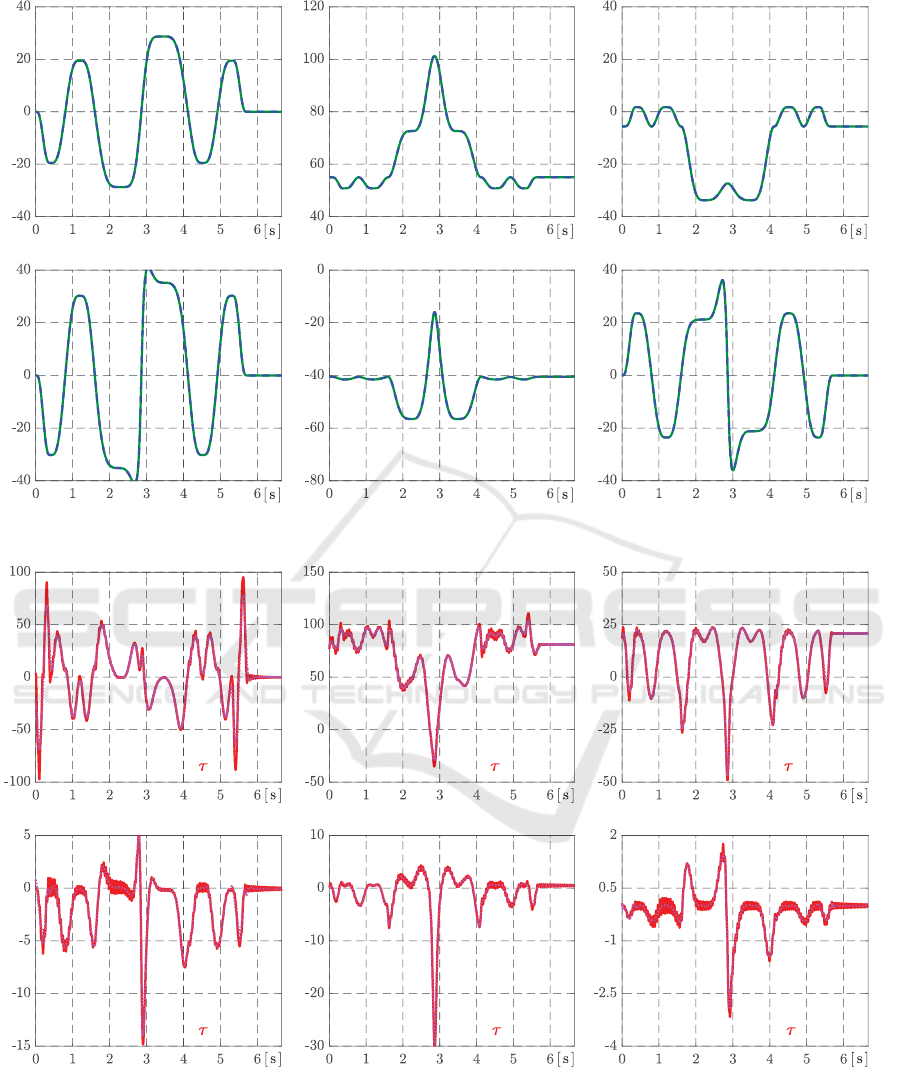
The Fig. 10 shows joint coordinates q

correspon-

ding to cartesian coordinates in Fig. 3. It is evi-

dent that the most difﬁcult motion phase is around

2.9 s, because the robot arms and end-effector are

in full motion speed and the trajectory decomposed

into the individual joint angles changes rapidly.

Fig. 11 shows corresponding situation in desig-

ned control actions τ

generated during control pro-

cess. Such rapid turn or change cause changes

in the model parameters, which cannot be expres-

sed with one linearized model (41) ﬁxed within re-

spective moving time intervals at standard design (39)

ICINCO 2018 - 15th International Conference on Informatics in Control, Automation and Robotics



t >@

G

tq



t >@

q

G

t



t >@

G

t



t >@

q

G

t



t >@

q

G

t



t >@q

G

t

Figure 10: Time histories of joint coordinates q

and their references q

: generalized coordinates q

i(·)

, i = 1, · · · , 6 .



t



>1P@



t



>1P@



t



>1P@



t



>1P@



t



>1P@



t



>1P@

Figure 11: Time histories of control actions: joint torques τ

, i = 1, · · · , 6 .

instead of varying nonlinear model along the same

time intervals at proposed nonlinear design based

on equations of predictions (25) and (26).

6 CONCLUSION

The proposed nonlinear design introduces speciﬁc

direct use of initial nonlinear continuous model wit-

Nonlinear Design of Model Predictive Control Adapted for Industrial Articulated Robots

hout any linearizaton and conventional model dis-

cretization. The introduced NdMPC can consider re-

asonable prediction horizon as regular MPC. Furt-

her emphasis will be placed on the selection analy-

sis of adequate numerical method, incremental offset-

free form and on a general point-to-point motion

in unconstrained and constrained robot workspace.

ACKNOWLEDGEMENT

This paper was supported by The Czech Academy of

Sciences, Institute of Information Theory and Auto-

mation.

REFERENCES

Arimoto, S. (1996). Control Theory of Non-linear Mecha-

nical Systems. Oxford Press.

Belda, K., B

ohm, J., and P

sa, P. (2007). Concepts of

model-based control and trajectory planning for pa-

rallel robots. In Proc. of the 13th IASTED Int. Conf.

on Robotics and Applications, pages 15–20.

Belda, K. and Novotn

y, P. (2012). Path simulator for ma-

chine tools and robots. In Proc. of MMAR IEEE Int.

Conf., pages 373–378, Poland.

Belda, K. and Rovn

y, O. (2017). Predictive control of 5

DOF robot arm of autonomous mobile robotic system

motion control employing mathematical model of the

robot arm dynamics. In 21st Int.Conf. on Process Con-

trol, pages 339–344.

Belda, K. and Vo

smik, D. (2016). Explicit generalized pre-

dictive control of speed and position of PMSM drives.

IEEE Trns. Ind. Electron., 63(2):3889–3896.

Belda, K. and Z

ada, V. (2017). Predictive control for offset-

free motion of industrial articulated robots. In Proc.

of MMAR IEEE Int. Conf., pages 688–693, Poland.

Butcher, J. (2016). Numerical Methods for Ordinary Diffe-

rential Equations. Wiley.

Chung, W., Fu, L., and Kr

oger, T. (2016). Motion Control,

pages 163–194. Springer.

Colombo, A. W., Karnouskos, S., Shi, Y., Yin, S., and

Kaynak, O. (2016). Industrial cyber-physical systems

scanning the issue. Proc. of the IEEE, 104(5):899–

903.

Faulwasser, T., Weber, T., Zometa, P., and Findeisen, R.

(2017). Implementation of nonlinear model predictive

path-following control for an industrial robot. IEEE

Tran. Control Syst. Technology, 25(4):1505–1511.

Franklin, G., Powell, J., and Workman, M. (1998). Digi-

tal Control of Dynamic Systems (3rd ed.). Addison

Wesley.

Groothuis, S., Stramigioli, S., and Carloni, R. (2017).

Modeling robotic manipulators powered by varia-

ble stiffness actuators: A graph-theoretic and port-

hamiltonian formalism. IEEE Trans. on Robotics,

33(4):807–818.

Houska, B., Ferreau, H., and Diehl, M. (2011). ACADO

toolkit – An open-source framework for automatic

control and dynamic optimization. Optimal Control

Applications and Methods, 32(3):298–312.

Kirches, C. (2011). Fast numerical methods for mixed-

integer nonlinear model-predictive control. Springer.

Kothare, M. V., Balakrishnan, V., and Morari, M.

(1996). Robust constrained model predictive con-

trol using linear matrix inequalities. Automatica,

32(10):13611379.

Lawson, C. and Hanson, R. (1995). Solving least squares

problems. Siam.

Maciejowski, J. (2002). Predictive Control: With Con-

straints. Prentice Hall.

Negri, G. H., Cavalca, M. S. M., and Celeberto, A. L.

(2017). Neural nonlinear model-based predictive con-

trol with faul tolerance characteristics applied to a ro-

bot manipulator. Int. J. Innovative Computing Infom-

ration and Control, 13(6):1981–1992.

Ordis, A. and Clarke, D. (1993). A state-space descrip-

tion for GPC controllers. J. Systems SCI., 24(9):1727–

1744.

Ostafew, C. J., Schoellig, A. P., Barfoot, T. D., and Col-

lier, J. (2016). Learning-based nonlinear model pre-

dictive control to improve vision-based mobile robot

path tracking. J. Field Robotics, 33(1):133–152.

Othman, A., Belda, K., and Burget, P. (2015). Physical mo-

delling of energy consumption of industrial articulated

robots. In Proc. of the 15th Int. Conf. on Control, Au-

tomation and Systems, pages 784–789, Korea. ICROS.

Siciliano, B., Sciavicco, L., Villani, L., and Oriolo, G.

(2009). Robotics – Modelling, Planning and Control.

Springer.

SPS IPC Drives (2017). Internationale fachmesse f

ur elek-

trische automatisierung, systeme und komponenten.

Online: < https://www.mesago.de/en/SPS/ >.

Wang, L. (2009). Model Predictive Control System Design

and Implementation Using MATLAB. Springer.

Wilson, J., Charest, M., and Dubay, R. (2016). Non-

linear model predictive control schemes with applica-

tion on a 2 link vertical robot manipulator. Robotics

and Computer-Integrated Manufacturing, 41:23–30.

ada, V. and Belda, K. (2017). Application of hamiltonian

mechanics to control design for industrial robotic ma-

nipulators. In Proc. of MMAR IEEE Int. Conf., pages

390–395, Poland.

Zanelli, A., Domahidi, A., Jerez, J., and Morari, M.

(2017). FORCES NLP: an efﬁcient implementation

of interior-point methods for multistage nonlinear

nonconvex programs. Int. J. Control, pages 1–17.

ICINCO 2018 - 15th International Conference on Informatics in Control, Automation and Robotics