Universal Translation Algorithm

for Formulation of Transport Network Problems

Anton Baldin, Kl

are Cassirer, Tanja Clees, Bernhard Klaassen,

Igor Nikitin, Lialia Nikitina and Inna Torgovitskaia

Fraunhofer Institute for Algorithms and Scientiﬁc Computing, Schloss Birlinghoven, 53754 Sankt Augustin, Germany

Keywords:

Complex Systems Modeling and Simulation, Non-Linear Systems, Applications in Energy Transport.

Abstract:

The formulation of transport network problems is represented as a translation between two domain speciﬁc

languages: from a network description language, used by network simulation community, to a problem de-

scription language, understood by generic non-linear solvers. A universal algorithm for this translation is

developed, an estimation of its computational complexity given, and an efﬁcient application of the algorithm

demonstrated on a number of realistic examples. Typically, for a large gas transport network with about 10K

elements the translation and solution of non-linear system together require less than 1 sec on the common hard-

ware. The translation procedure incorporates several preprocessing ﬁlters, in particular, topological cleaning

ﬁlters, which accelerate the solution procedure by factor 8.

1 INTRODUCTION

This short paper continues our previous work (Clees

et al., 2016), where we discuss a general possibil-

ity for formulation of transport network problems as

a translation between two abstract representations,

a human-readable network description and a solver-

speciﬁc code. This approach provides an open type of

modeling, where both the network description and the

physical laws deﬁning the transport are completely in

the hands of the user and can be given as plain text

ﬁles. There is a universal translation procedure con-

verting them to a problem description suitable for a

given solver. In this approach one is not bound to any

particular program and is ﬂexible in the choice and

experimentation with different solution kernels.

In state of the art, the solution of transport net-

work problems combines well established model-

ing approaches with the standard solvers of non-

linear systems. The network applications vary by the

types of transported media: water supply (Rogalla

and Wolters, 1994; Stevanovic et al., 2009), elec-

tric power transmission (Milano, 2015; Zimmerman

and Murillo-Sanchez, 2015), gas transport networks

(Scheibe and Weimann, 1999; Aymanns et al., 2008),

etc. For each of them different types of network prob-

lems can be formulated: stationary, dynamical, feasi-

bility, optimization, optimal control. All these prob-

lems can be represented in terms of non-linear pro-

gramming (NLP), for which powerful solution algo-

rithms are available (Bazaraa and Shetty, 1979; Bert-

sekas, 1999; Avriel, 2003; Fletcher, 2013). The algo-

rithms are implemented in various software packages:

MINOS (Murtagh and Saunders, 1978), SNOPT (Gill

et al., 2005), IPOPT (W

achter and Biegler, 2006),

KNITRO (Nocedal and Wright, 2006), COUENNE

(Belotti et al., 2013). None of the approaches, how-

ever, provides a universal algorithm for formulation

of transport network problem which would be inde-

pendent on the type of trasport media and a particular

solver.

In spite of the variety of different possibilities,

there is a common way of formulating the network

problems, based on the fact that the network descrip-

tions for all types are quite uniform. The networks

are given as graphs with the properties, assigned per

element. The physical laws, describing the propaga-

tion of properties over the graph, are given as equa-

tions and inequalities, assigned per element type. The

equations can be written in the syntax of the tar-

get solver, e.g., in a form of expression trees (Gay,

2005) or a human-readable syntax of higher level sys-

tems, such as AMPL, Modelica, Mathematica, Mat-

lab. Considering the network description as an ab-

stract text and the list of physical laws as a dictionary,

one can represent the problem formulation as a trans-

Baldin, A., Cassirer, K., Clees, T., Klaassen, B., Nikitin, I., Nikitina, L. and Torgovitskaia, I.

Universal Translation Algorithm for Formulation of Transport Network Problems.

DOI: 10.5220/0006831903150322

In Proceedings of 8th International Conference on Simulation and Modeling Methodologies, Technologies and Applications (SIMULTECH 2018), pages 315-322

ISBN: 978-989-758-323-0

315

lation procedure between two formal languages (Har-

rison, 1978).

In the present paper we will describe an imple-

mentation of this idea, give detailed estimations of

computational complexity, present several realistic

examples and the results of performance tests. We

will also discuss the aspects of multiphase solution

procedure and a coupling of multiple network sectors.

The translation procedure is straightforwardly imple-

mentable and highly parallelizable, allowing separate

processing per every element.

In Section 2 the main translation algorithm is pre-

sented, its functionality is demonstrated on a simple

example of the water supply network and its compu-

tational complexity is estimated. In Section 3 the ﬁl-

ters are described, implementing the necessary pre-

and postprocessing steps. In Section 4 several real-

istic examples are considered and the results of the

corresponding performance tests are given.

2 THE ALGORITHM

The network (NET) is described by a set of elements,

each of them is a set of properties, each speciﬁed by

a map from the property name to the property value,

of the form prop=val. The names and values can be

generally represented as character strings.

Translation matrix (TM) is a set of rules deﬁning

variables and equations, applied when the elements

match a speciﬁed pattern. The pattern is given also

as a set of properties of the form prop=val. If this

set is a subset of properties in the element, the rule is

applied to the element.

The rules deﬁning the variables have a form

var=prop. When the rule is applied, a new variable

is introduced and the property prop=v

is inserted

in the given element.

The rules deﬁning the equations have a form

eq=expr, where expr contains a mathematical for-

mula for the equation in the target syntax. The for-

mula has constant, non-modiﬁable parts and variable

parts. The variable parts are marked up by square

brackets, containing the property names, in the form

[prop]. When the rule is applied, the property is

found in the given element, replaced by the corre-

sponding val and the brackets are removed. As a re-

sult, the corresponding variables and constants from

the given element become substituted into the equa-

tion. Algorithmically, this can be done as follows.

Algorithm (universal translator):

variables:

foreach element in NET

for all matching var prototypes in TM

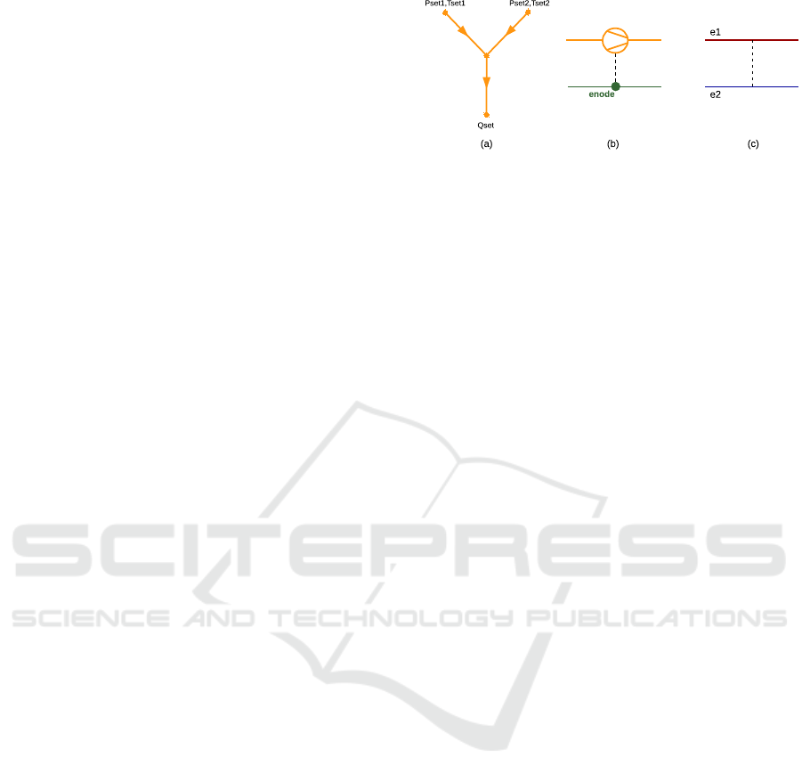
Figure 1: Examples of networks. From left to right: simple

water network with three pipes, coupling between the edge

in gas network and the node in power network, coupling

between two edges.

define variables (v0,v1,...)

put them to element (prop=v0,...)

equations:

foreach element in NET

for all matching eq prototypes in TM

find [props] in element description

substitute their vals into the equation

stream the equation

Let us show the work of the algorithm on the fol-

lowing example. The test network is displayed on

Fig. 1 left. It is intentionally simple, for illustration

purposes.

Example 1.1: water network (NET)

# nodes

class=n,name=n1,type=pset,pset=7

class=n,name=n2,type=pset,pset=5

class=n,name=n3,type=demand

class=n,name=n4,type=qset,qset=30

# edges

class=e,name=p1,type=p,node1=n1,node2=n3,R=0.3

class=e,name=p2,type=p,node1=n2,node2=n3,R=0.05

class=e,name=p3,type=p,node1=n3,node2=n4,R=0.1

The network description contains topological rep-

resentation of the graph in the form of connections

(node1,2). It also speciﬁes water supply pressures

(psets), output ﬂow (qset) and hydraulic resistances

of the pipes (R).

Example 1.2: translation matrix for water networks

with laminar ﬂow (TM)

# variables with start values

class=n, var=P, var0=1

class=e, type=p, var=Q, var0=0

# Kirchhoff law

class=n, type=demand, eq="[sumadj][Q]"

class=n, type=qset, eq="[sumadj][Q]-[qset]"

class=n, type=pset, eq="[P]-[pset]"

# equations of elements (linear resistors)

class=e, type=p,

eq="[P@node1]-[P@node2]-[R]*[Q]"

SIMULTECH 2018 - 8th International Conference on Simulation and Modeling Methodologies, Technologies and Applications

316

The translation matrix introduces for every node

(class=n) the pressure variable P with the starting

value 1, for every pipe (class=e, type=p) the ﬂow vari-

able Q with the starting value 0. The equations in-

corporate Kirchhoff law written for every node. It

is represented by an operator [sumadj], implement-

ing a sum of ﬂows in edges adjacent to a given node,

with the signs speciﬁed by the incidence matrix of the

graph:

[sumadj][Q]

∑

. (1)

The incidence matrix I is internally evaluated using

given connectivity data. The other equations describe

linear pressure drops according to the given resis-

tances. A reference operator is used to deﬁne pressure

in end nodes: [P@node1,2].

The application of translation algorithm gives the

following output.

Example 1.3: water network problem (PRO)

7 7 #nvars,neqs

v0-7 #eq0

v1-5 #...

v4+v5-v6

v6-30

v0-v2-0.3*v4

v1-v2-0.05*v5 #...

v2-v3-0.1*v6 #eq6

This is the list of the equations (represented by

their left hand sides). It is ready for solution by such

solvers as Mathematica and Matlab, accepting the ex-

pressions in human readable form. The equations can

be also retranslated in the other formats, suitable for a

particular solver. Here are the same equations in NLP

format (explained further in Sec. 3.3).

Example 1.4: water network problem (NLP)

7 7 #nvars,neqs

o1 v0 7 #eq0

o1 v1 5 #...

o54 3 v4 v5 o16 v6

o1 v6 30

o1 o1 v0 v2 o2 0.3 v4

o1 o1 v1 v2 o2 0.05 v5 #...

o1 o1 v2 v3 o2 0.1 v6 #eq6

The solver returns the answer, which can be

mapped again to the NET form.

Example 1.5: water network problem solution

name=n1,P=7

name=n2,P=5

name=n3,P=4

name=n4,P=1

name=p1,Q=10

name=p2,Q=20

name=p3,Q=30

Complexity estimation for the algorithm is

O(Nelem Nprop Neq), where Nelem – number of el-

ements, Nprop – number of properties per element,

Neq – number of equations per element. It is identi-

cal with the complexity of matrix multiplication

NET * TM = PRO (2)

where NET(Nelem,Nprop), TM(Nprop,Neq),

PRO(Nelem,Neq) are matrices of given dimensions.

If the problem had only one type of elements and

were linear, it were really speciﬁed by a matrix

multiplication with the operations count given above.

For non-linear problems the same estimation with

average values holds, Nprop – average number of

properties per equation, Neq – average number of

equations per element.

It is important to note that a particular represen-

tation of NET and TM structures as a simple list of

properties, e.g., NetList (Clees et al., 2016) or in other

format plays no role for the algorithm. These formats

are different implementations for the same abstract

structure (sets of maps) used to represent the network.

On the implementation level, the readers of NET and

TM have to be separated from the algorithms work-

ing on abstract structures, which can be conveniently

represented by set and map containers of C++ Stan-

dard Template Library (STL). This allows to use ef-

ﬁcient search and set-theoretical algorithms available

in STL. On the other hand, the syntax of TM is ﬂex-

ible and is completely in user hands. One can deﬁne

the other names for the properties in NET and adopt

TM accordingly. One can also change the syntax of

the equations in TM according to the solver language.

In this way the format independence of the main al-

gorithm is achieved.

The translation algorithm is highly parallelizable.

The processing loops can be per-element separated

and proportionally accelerated by the usage of mul-

tiprocessor architectures.

3 THE FILTERS

The network description often requires an additional

preprocessing. Also an adaptation to a particular

solver can be necessary. This can be done by spe-

cialized modules for ﬁltering the data.

3.1 Topological Filters

Topological cleaning ﬁlters are required for the net-

works containing subgraphs disconnected from any

source. For instance, in gas and water networks, such

sources are pressure and temperature supplies (Pset,

Universal Translation Algorithm for Formulation of Transport Network Problems

317

Tset). Also the elements with vanishing or small re-

sistance bear a problem. The loops formed from such

elements have unstable ﬂow balance. In both cases

the corresponding network problems are ill-deﬁned

and can lead to a solver failure. Topological clean-

ing ﬁlters can recognize such parts and remove them

at an early stage.

Topological reduction ﬁlters provide a deeper net-

work optimization. When the edge elements are de-

scribed by physical proﬁles, entering into the element

equations, their serial and parallel connections also

possess a computable common physical proﬁle. Tree-

like connections with given ﬂows (Qsets) in the leaves

can be contracted to the root with a single Qset. These

operations are encountered in theory of generalized

series-parallel graphs (SPG/GSPG), (Eppstein, 1992;

Korneyenko, 1994) and their practical application al-

lows to reduce the networks signiﬁcantly, by a factor

upto 100 (Clees et al., 2018b).

3.2 Classiﬁcation Filters

The particular applications should decide which ele-

ments belong to nodes, edges (class=n,e) as necessary

for the work of topological ﬁlters, Kirchhoff sum op-

erator, etc. Additional classiﬁcation could be neces-

sary. For instance, in gas transport networks the deci-

sion, whether a node is Pset, is taken on the basis of a

complicated logic, involving the presence of gas com-

position (gasmix). This evaluation can be spared for

the main translation module and transferred to a spe-

cialized ﬁlter. Other examples of classiﬁcation will be

given below in Section 4.

3.3 Retranslation Filters

Particular solvers can require a special coding, differ-

ent from human readable form suitable for TM. For

instance, such solvers as IPOPT, SNOPT, MINOS use

special NLP input (Gay, 2005), based on Polish preﬁx

notation (PPN) of all formulae and a uniﬁed encod-

ing of all variables, numerical constants and opera-

tors. Using a quadratic pipe law as an example (Clees

et al., 2016):

pow(P@node1,2)-pow(P@node2,2)-R*Q*abs(Q)=0

written in PPN form:

- - pow P@node1 2 pow P@node2 2 * * R Q abs Q

using encoding rules:

P@node1 P@node2 Q R 2

v1 v2 v3 n0.1 n2

pow abs * -

o5 o15 o2 o1

one obtains an equivalent expression:

o1 o1 o5 v1 n2 o5 v2 n2 o2 o2 n0.1 v3 o15 v3

In the same way all equations in the system have to

be encoded. An important observation is that such

encoding becomes much more efﬁcient when applied

to TM rather than to PRO, see Figure 2. It is simi-

lar to retranslating a short dictionary to another lan-

guage and its usage for the translation of a long doc-

ument. The complexity of direct retranslation of the

problem increases linearly with the size of network,

as O(NET ), while the performance of retranslation

of TM depends only on its size, as O(T M), which is

much faster in practical applications.

In our implementation, the retranslation is done by

a specialized ﬁlter preNLP. When applied to TM, the

bracketed [prop] parts are left unchanged and used

further for direct substitution by the main translation

algorithm utrans. Certain postprocessing operations

are also required, such as inserting a header, form-

ing a structural Jacobian, providing starting point,

etc. They are done by the postNLP ﬁlter, as shown

schematically in Figure 2.

4 EXAMPLES OF USAGE

4.1 Multiphase Problems

Figure 3 top shows a typical one-phase solution pro-

cedure. The necessary translation is done once, the

result is passed to the NLP solver and the answer is

again encoded to NET form with the x2net ﬁlter.

The applications can require multiple phases, e.g.,

distribution of ﬂows in the water network can be used

to compute the temperature distribution.

Example 2.1: water network description for tempera-

ture mix

# nodes

class=n,name=n1,ttype=tset,tset=280

class=n,name=n2,ttype=tset,tset=300

class=n,name=n3,ttype=demand

class=n,name=n4,ttype=demand

# edges

class=e,name=p1,node1=n1,node2=n3,

Q=10,qtype=1,in=n1

class=e,name=p2,node1=n2,node2=n3,

Q=20,qtype=1,in=n2

SIMULTECH 2018 - 8th International Conference on Simulation and Modeling Methodologies, Technologies and Applications

318

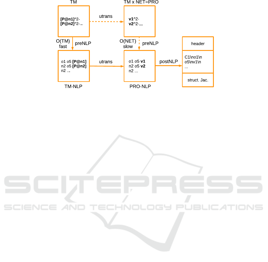
Figure 2: Retranslation of the problem to NLP form. The translation path, shown by solid lines, is much faster than the one

shown by dashed lines.

class=e,name=p3,node1=n3,node2=n4,

Q=30,qtype=1,in=n3

Example 2.2: translation matrix for temperature mix

in water networks

# variables

class=n, var=T

class=e, var=T

# equations

class=n, ttype=tset, eq="[T]-[Tset]"

class=n, ttype=demand, eq="[summix][Q][T]-[T]"

class=e, qtype=1, eq="[T]-[T@in]"

class=e, qtype=0,

eq="[T]-([T@node1]+[T@node2])/2"

In the corresponding workﬂow, displayed on Fig-

ure 3 bottom, the classiﬁcation ﬁlter wtmix is used

to set in NET ttype ﬁelds at nodes, qtype and in

ﬁelds at edges. In TM the temperature variables are

assigned to nodes and edges. The ﬁeld ttype is used

to distinguish between the temperature sources and

intermediate nodes. In the intermediate nodes an op-

erator [summix] implements a mixture of the temper-

ature from the adjacent edges with the weights de-

pending on the ﬂows:

[summix][Q][T]

∑

, (3)

= u

∑

, u

= max(I

,0).

It is similar to [sumadj] operator, but effectively in-

volves only incoming ﬂows with I

> 0 and uses

them for weighting. The physical meaning of the mix

equation is that the weighted sum of incoming tem-

peratures in edges equals to the temperature in the

node.

In the edge the temperature is generally (qtype=1)

deﬁned as the temperature in the upstream node T@in.

The exception is zero ﬂow case (qtype=0), where the

half-sum of temperature at end nodes is taken. This is

done to regularize the problem in subgraphs with zero

ﬂows. The ﬁelds qtype and in are set by the wtmix

ﬁlter using the available ﬂow distribution.

The resulting problem in the second phase is linear

and is solved in one iteration by the solver.

Example 2.3: water temperature mix solution

name=n1,T=280

name=n2,T=300

name=n3,T=293.33

name=n4,T=293.33

name=p1,T=280

name=p2,T=300

name=p3,T=293.33

4.2 Multisectoral Problems

The concept of universal translation can be naturally

extended to process the networks with multiple sec-

tors, also with coupling between them.

Example 3: translation matrix for multisectoral cou-

pling

# variables

class=n, sector=gas, var=P

class=e, sector=gas, var=Q

class=n, sector=water, var=P

class=e, sector=water, var=Q

class=n, sector=power, var=U

class=e, sector=power, var=I

...

# equations

class=e, sector=gas, type=p,

eq=[P@node1]*abs([P@node1])

-[P@node2]*abs([P@node2])

-[R]*[Q]*abs([Q])

class=e, sector=power, type=r,

Universal Translation Algorithm for Formulation of Transport Network Problems

319

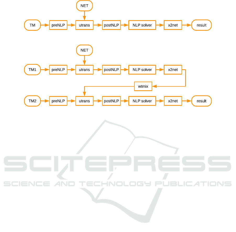
Figure 3: Solution workﬂows: one-phase on the top, two-phase at the bottom.

eq=[U@node1]-[U@node2]-[R]*[I]

class=e, sector=water, type=p,

eq="[P@node1]-[P@node2]-[R]*[Q]"

class=e, sector=gas, type=c, drive=E,

eq=[Q]

-efun([P@node1],[P@node2],[U@enode])

...

Here three sectors (gas, power, water) are intro-

duced. The coupling between power and gas is im-

plemented using a cross-referencing. The typical net-

work is shown on Figure 1 middle. The compressor

element in the gas network has an equation, depend-

ing on the voltage variable [U@enode] in the node

of the power network. For the reference the ﬁeld

[enode] in the compressor is used. Similar construc-

tion can be used to deﬁne the coupling between edge

elements, as shown on Figure 1 right, for modeling of

heat exchangers, power transformers, etc.

4.3 Realistic Network Problems

For the validation, we have applied the developed al-

gorithms for solving a number of realistic network

problems, received from our industrial partners. The

smallest test cases are shown on Figure 4. The gas

transport network N1, shown in the top image, con-

tains about a hundred of nodes and edges, has two

Pset supplies (shown by rhombi) and three Qset ex-

its (n76, n80, n91, shown by triangles). The bottom

image shows a water cooling network NSR/KLT72

of comparable complexity. The other, medium-sized

gas network N2 contains about a thousand nodes and

edges, while the largest considered gas network N3

has about ﬁve thousand nodes and edges.

To assess the performance of the algorithm, we se-

lect as a measure the timing of translation and solution

steps for the networks of different complexity. The

results of the tests are collected in Table 1. Solution

for these gas networks is performed in two phases.

First, all compressors and regulators are set in special

mode with their goals enforced, providing linear ele-

ment equations. The result is used as a starting point

for the second phase, with compressors and regula-

tors set to their actual element equations. The solution

can be also done in one phase but the solution in two

phases appears to be empirically faster. The timing in

the table is given per one phase.

In comparison with our previous numerical exper-

iments (Clees et al., 2018a), the translation procedure

now includes topological cleaning algorithms, which

for the largest network N3 accelerate the solver pro-

cedure by a factor about 8. With this acceleration the

solver procedure now requires a CPU time compara-

ble with the translation time.

In more details, the gas compressors in these tests

were considered in frames of the so called free model.

In this model the compressors attempt to satisfy spec-

iﬁed goals, such as ﬁxed output pressure or through-

put ﬂow, while the restrictions on revolution number

and power of the drive are not imposed. Considera-

tion of these restrictions is possible in frames of the

advanced model (Clees et al., 2018b). Its implemen-

tation requires an additional ﬁlter, transforming indi-

vidual characteristics of the compressor to tabulated

functions, representing the extended element equa-

tion.

Further, the tests were performed with a gas of

constant composition and temperature. Implementa-

tion of the mix procedure for gas is analogous to the

SIMULTECH 2018 - 8th International Conference on Simulation and Modeling Methodologies, Technologies and Applications

320

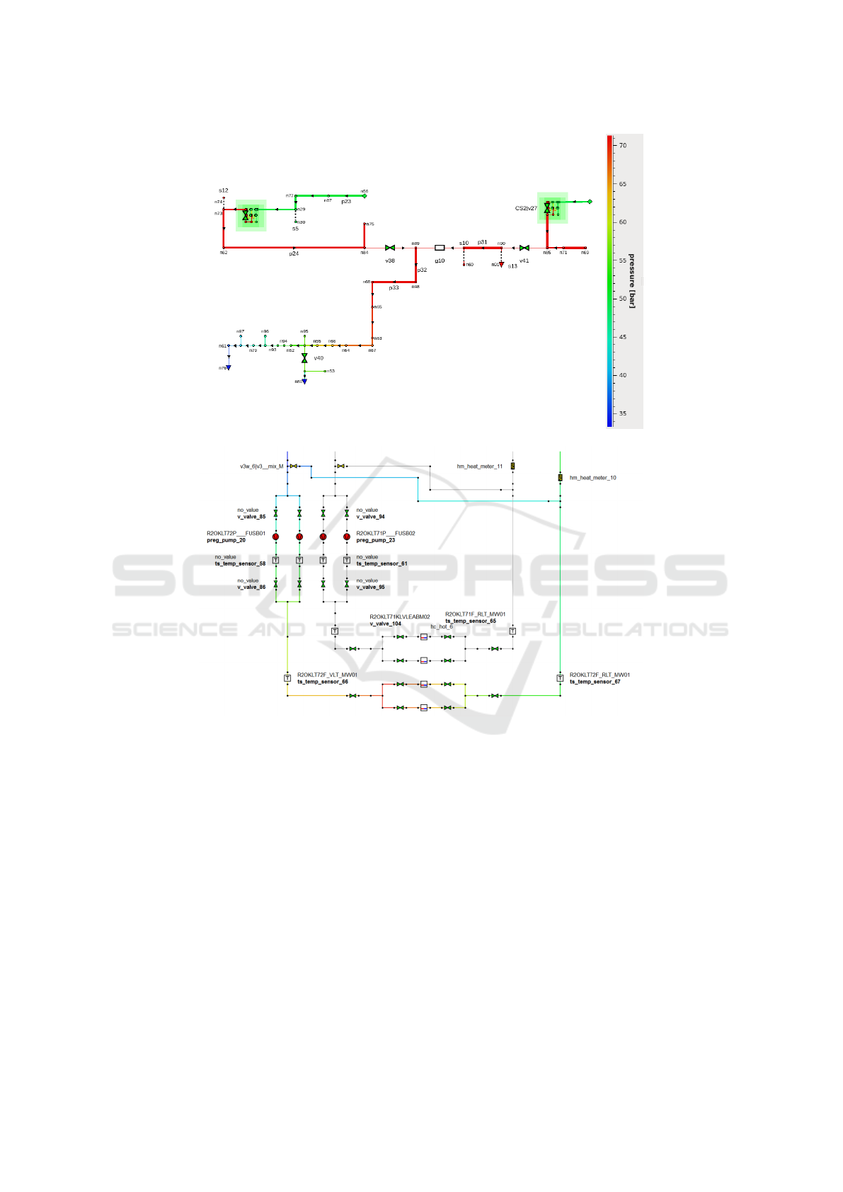
Figure 4: Realistic test networks: gas network N1 on the top, water cooling network NSR/KLT72 at the bottom.

above described mix step for water networks, requir-

ing to upgrade the solution procedure by one more

phase. The implementation of the gas mix phase and

the advanced model of compressors is on the way.

5 CONCLUSIONS

We have presented the formulation of transport net-

work problems as a translation between two formal

languages. As input one has a network description

in a form of a graph with properties and a conﬁg-

urable set of translation rules, corresponding to physi-

cal equations of transport, given per element type. As

output one has a problem description given as a sys-

tem of non-linear equations in a form, suitable for the

chosen solver.

A universal translation algorithm has been devel-

oped, possessing computational complexity linear in

the number of elements in the graph, the number of

properties per element and the number of equations

per element type. The processing can be separated

element-wise and allows massive parallelization.

A number of realistic examples has been used to

test operability and performance of the algorithm, in-

cluding water supply, cooling circuits, gas transport,

power networks, as well as multisectoral couplings.

Typically, for a large gas transport network with about

10K elements the translation and solution of non-

linear system together require less than 1 sec. The

translation procedure incorporates several preprocess-

ing ﬁlters, in particular, topological cleaning ﬁlters,

Universal Translation Algorithm for Formulation of Transport Network Problems

321

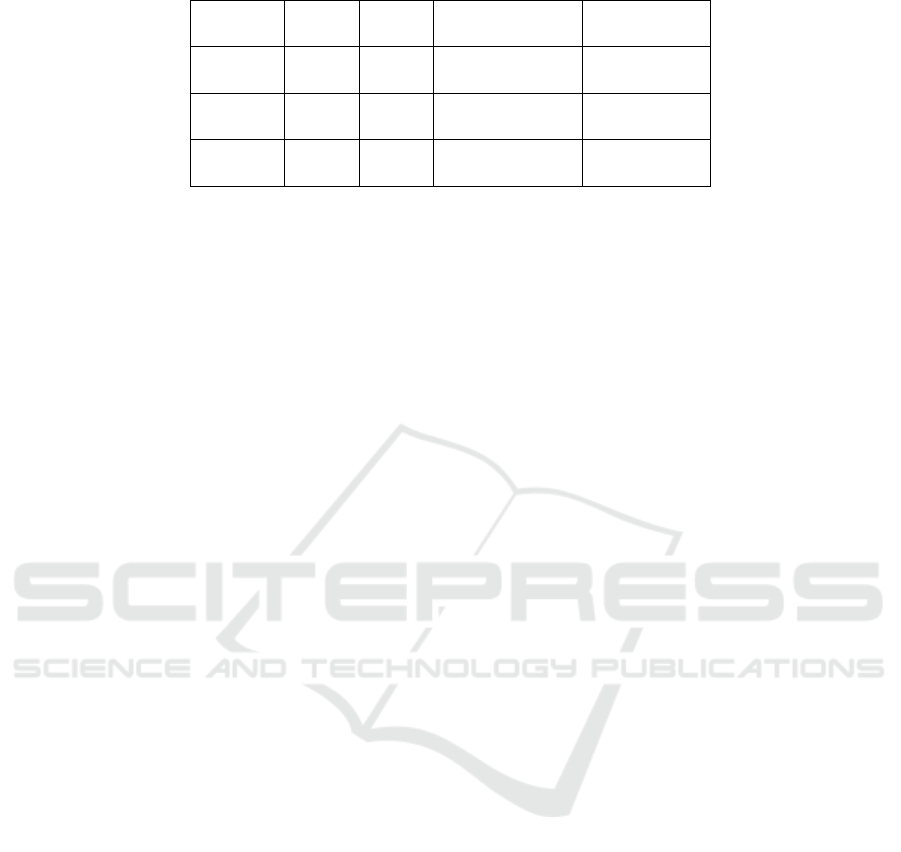
Table 1: Performance of translation and solution phases for various networks.

network nodes edges translation, sec solution, sec

N1 100 111 0.04 0.02

N2 931 1047 0.15 0.24

N3 4466 5362 0.39 0.42

(timing for 3 GHz Intel i7 CPU 8 GB RAM workstation)

which accelerate the solution procedure by factor 8.

Currently we are working on the extension of the

translation procedure by the advanced modeling of

gas compressors and mix phase for gas composition

and temperature. Our further plans include the accel-

eration of the solver procedure by applying topologi-

cal reduction algorithms and parallelization of trans-

lation procedure on multiprocessor architectures.

ACKNOWLEDGMENTS

This work is supported by German Federal Ministry

for Economic Affairs and Energy, project BMWI-

0324019A, MathEnergy: Mathematical Key Tech-

nologies for Evolving Energy Grids. This material is

also based upon work supported by the German Bun-

desland North Rhine-Westphalia using fundings from

the European Regional Development Fund, grant Nr.

EFRE-0800063, project ES-FLEX-INFRA.

REFERENCES

Avriel, M. (2003). Nonlinear Programming: Analysis and

Methods. Dover Publishing.

Aymanns, P. et al. (2008). Online simulation of gas dis-

tribution networks. 9th SIMONE Congress, October

15–17, 2008, Dubrownik, Croatia.

Bazaraa, M. S. and Shetty, C. M. (1979). Nonlinear pro-

gramming: theory and algorithms. John Wiley &

Sons.

Belotti, P. et al. (2013). Mixed-integer nonlinear optimiza-

tion. Acta Numerica, 22:1–131.

Bertsekas, D. P. (1999). Nonlinear Programming. Athena

Scientiﬁc.

Clees, T. et al. (2016). MYNTS: Multi-phYsics NeTwork

Simulator. In SIMULTECH 2016, July 29–31, 2016,

Lisbon, Portugal, pages 179–186. SCITEPRESS.

Clees, T. et al. (2018a). Making Network Solvers Glob-

ally Convergent. Advances in Intelligent Systems and

Computing, 676:140–153.

Clees, T. et al. (2018b). Modeling of Gas Compressors

and Hierarchical Reduction for Globally Convergent

Stationary Network Solvers. International Journal On

Advances in Intelligent Systems, IARIA (submitted).

Eppstein, D. (1992). Parallel recognition of series-parallel

graphs. Information and Computation, 98:41–55.

Fletcher, R. (2013). Practical Methods of Optimization.

John Wiley & Sons.

Gay, D. M. (2005). Writing .nl Files. Technical Report,

Sandia National Laboratories, Albuquerque.

Gill, P. E. et al. (2005). SNOPT: An SQP algorithm for

large-scale constrained optimization. SIAM Review,

47(1):99–131.

Harrison, M. A. (1978). Introduction to Formal Language

Theory. Addison-Wesley.

Korneyenko, N. M. (1994). Combinatorial algorithms on

a class of graphs. Discrete Applied Mathematics,

54:215–217.

Milano, F. (2015). PSAT Software. faraday1.ucd.ie/psat

.html.

Murtagh, B. and Saunders, M. (1978). Large-scale lin-

early constrained optimization. Mathematical Pro-

gramming, 14:41–72.

Nocedal, J. and Wright, S. J. (2006). Numerical Optimiza-

tion. Springer.

Rogalla, B.-U. and Wolters, A. (1994). Slow transients

in closed conduit ﬂow – part I: Numerical meth-

ods. In Chaudhry, M. H. and Mays, L. W., editors,

Computer Modeling of Free-Surface and Pressurized

Flows, volume 274 of NATO ASI Series, pages 613–

642. Springer, Netherlands.

Scheibe, D. and Weimann, A. (1999). Dynamische Gas-

netzsimulation mit GANESI. GWF Gas/Erdgas,

(9):610–616.

Stevanovic, V. D. et al. (2009). Prediction of thermal tran-

sients in district heating systems. Energy Conversion

and Management, 50(9):2167–2173.

achter, A. and Biegler, L. T. (2006). On the implemen-

tation of an interior-point ﬁlter line-search algorithm

for large-scale nonlinear programming. Mathematical

Programming, 106(1):25–57.

Zimmerman, R. D. and Murillo-Sanchez, C. E. (2015).

Matpower 5.1 User’s Manual. www.pserc.cornell.

edu/matpower.

SIMULTECH 2018 - 8th International Conference on Simulation and Modeling Methodologies, Technologies and Applications

322