Flexibility Definition for Smart Grid Cells in a Decentralized Energy
System
Helen Sawall, Andreas Scheuriker and Daniel Stetter
Fraunhofer Institute for Industrial Engineering IAO, Stuttgart, Germany
University of Stuttgart IAT, Stuttgart, Germany
Keywords:
Load Balancing in Smart Grids, Scheduling and Switching Power Supplies, Architectures for Smart Grids.
Abstract:
The networking of individual cells to form a decentralised network represents a possible approach for an
energy system of the future, which is up to the challenges of the energy transition, such as stochastic electricity
generation through renewable energies and the participation of many small producers. In this context, the
sharing of flexibility in load profiles of cells requires a uniform definition to create a communication basis. This
paper presents a generic description of flexibility by defining the latter as the set of all possible and permissible
load profiles, taking into account dependencies between plants, technical constraints and maintaining energy
balance within networks. The resulting solution space for load optimization problems, in form of the flexibility
of a cell, can be described as a partial set of the R
p·T
by derived constraints. The solution space is the keystone
for further flexibility communication.
1 INTRODUCTION
In addition to the expansion of renewable energy re-
sources and their integration into the existing electri-
city supply as well as the increase in energy efficiency,
the energy turnaround comes along with a bundle of
other key challenges. Besides questions concerning
investment distribution, resource conservation, social
acceptance and political implementation, the focus is
above all on the appropriate expansion of the energy
infrastructure (Mauser, 2017). A concentration on the
pure expansion of grid capacity, for example through
the construction of new high-voltage lines from nort-
hern to southern Germany, does not meet this chal-
lenge entirely. Alternative options such as intelligent
load and application management of energy (Palen-
sky and Dietrich, 2011) and the use of storages are in-
dispensable. In this context, there is talk of smart grid
architectures (Greer et al., 2014), energy management
systems (Allerding et al., 2014), smart energy storage
and demand side management (Gottwald et al., 2011).
What all these concepts have in common is that they
examine approaches to solutions based on intelligent
use of information and data as well as their provision
and exchange.
An example for the development and demonstra-
tion of a smart grid approach which is supposed to re-
present the blueprint for a cellularly structured
energy system of the future in Southern Germany is
the SINTEG project C/sells (Smart Grids-Plattform
Baden-W
¨
urttemberg e.V, 2017). The networking
of energy units, denoted as cells, is intended to
create a secure and above all robust and resilient
energy infrastructure that can cope with the new
requirements of a decentralised supply system with
many small generators, greater complexity and
stochasticity due to for the greatest part volatile
renewable energies. This is to be done on the basis
of the use of flexibility in the load profiles of initially
individual cells and in a further step across cells.
Since individual cells differ greatly in their structure,
i.e. the energy-generating and consuming plants
contained in them, a generic definition of flexibility
is necessary as a basis for communication. Such a
definition and further steps to operate the system as
a whole is developed in this paper. The basic idea
is to describe flexibility in its most general form as
the set of all possible and permissible load profiles
for a future time window. To determine this set,
technical grid and plant restrictions, dependencies
on energy flows over time and energy balance
aspects within grids must be taken into account.
In addition to its generic nature, the main criteria
for the definition presented here were the suitability to
130
Sawall, H., Scheuriker, A. and Stetter, D.
Flexibility Definition for Smart Grid Cells in a Decentralized Energy System.
DOI: 10.5220/0006803401300139
In Proceedings of the 7th International Conference on Smart Cities and Green ICT Systems (SMARTGREENS 2018), pages 130-139
ISBN: 978-989-758-292-9
Copyright
c
 2019 by SCITEPRESS – Science and Technology Publications, Lda. All rights reserved

describe a solution space for optimization problems
of load profiles as well as the possibility to consider
different energy sources, controllable and uncontrol-
lable plants and storages.
2 RELATED WORK
In order to overcome the hurdles of energy system
transition, it is not sufficient to consider each cell
(energy unit) individually. In addition to the inter-
nal use of flexibilities in the load profile, a network-
wide communication between individual cells is also
necessary. The networking of the cells allows joint
action, which supports and promotes the development
and maintenance of a secure and robust energy infra-
structure, eventually yielding both system adequacy
and security. In order to create a communication ba-
sis, it is necessary in a first step to develop a generic
definition of flexibility, which can be applied to a wide
variety of contexts and cells. Therefore, we will now
present our basic criteria (C1-C7) for such a defini-
tion:
C1 Applicability to different cells with various con-
trollable and non-controllable plants, as well as
the possibility to integrate flexibilities of subordi-
nate cells into higher-level cells.
C2 Suitability as solution space for a subsequent op-
timization of load.
C3 Possibility to take into account the temporal load
profiles of individual plants.
C4 Possibility of modelling loads at plant level.
C5 Consideration of energy storage systems.
C6 Implementability within the scope of a load opti-
mization.
C7 Possibility of optimization according to different
criteria.
In addition to these basic criteria, we identified
ten concrete requirements (R1-R10) indicated in Ta-
ble 1 which utterly describe our model as presented in
section 3.2.
In 1985 Gellings presented his formulation of de-
mand side management (Gellings, 1985). His work
is not the concrete concept for defining flexibility for
interoperable energy systems although modern solu-
tions are mostly based on his ideas.
In 2011 the European Commission and EFTA
issued the Smart Grid Mandate M/490 to the three
European Standard Organizations (ESOs), CEN,
CENELEC and ETSI which requests them to de-
velop a framework to enable a continuous standard
Table 1: Requirements for a mathematical definition of flex-
ibilities.
Requirement Formulation
R1 Energy conservation principle
for networks
R2 Physical limit constraints
R3 Specified power at specified ti-
mes
R4 Dependencies over time
R5 Dependencies between plants
R6 Dependencies on stochastic en-
vironmental influences
R7 Number of total operation hours
R8 Specified energy at specified ti-
mes
R9 Specific switch-on and switch-
off times
R10 Energy conservation principle
for plants
enhancement and development in the smart grid
field. In order to fulfill the requested work the ESOs,
together with the relevant stakeholders, established
the CEN-CENELEC-ETSI Smart Grid Coordination
Group (SG-CG), being responsible for coordinating
the ESOs reply to M/490. In this context, the latter
association adopted the following non-technical
definition of flexibility:
”On an individual level, flexibility is the modifi-
cation of generation injection and/or consumption
patterns in reaction to an external signal (price
signal or activation) in order to provide a service
within the energy system. The parameters used
to characterize flexibility in electricity include: the
amount of power modulation, the duration, the rate of
change, the response time, the location etc.” (Smart
Grid Coordination Group, 2014)
This understanding of flexibility, as the use of ex-
isting leeway, is not appropriate for the context con-
sidered here, in which the ultimate goal is to identify
optimal load profiles. In order to enable an optimi-
zation of the latter mentioned in a subsequent step, it
is first necessary to describe flexibility as the set of
all possible/permissible load profiles in an energy sy-
stem. In addition, flexibility should be defined inde-
pendently of external signals, since external price or
activation signals do not change the number of possi-
ble load profiles.
In many areas, there are already very different
energy management systems (EMS) in place today.
These support and take over the energy, charge and
load management for small units such as smart resi-
Flexibility Definition for Smart Grid Cells in a Decentralized Energy System
131

Table 2: Requirements for a mathematical definition of flexibilities.
Source C1 C2 C3 C4 C5 C6 C7 Requirements
(Gellings, 1985) no no no no no no no -
(Weckmann et al.,
2017)
no no no no no yes no -
(Khoury et al., 2016) no yes in part no yes yes in part R1, R2, R3,
R8, R9
(Mauser et al., 2016) in part yes yes yes yes yes yes R1-R5, R10
(Tushar et al., 2014) no no no no in part yes no -
(Liu et al., 2014) no yes in part in part no yes no R1, R2, R4
(Liu et al., 2015) no yes in part in part no yes no R2, R4
dential buildings (Khoury et al., 2016) up to compa-
nies (Weckmann et al., 2017) and entire infrastructu-
res such as airports.
Due to the growing importance of EMS, there is
also a large number of publications on this subject
which have been considered in the search of a suit-
able flexibility definition.
(Weckmann et al., 2017) pursue the goal to ensure a
stable and cost efficient energy supply in industrial
energy systems where flexibilities are strongly limi-
ted by ensuring the production performance. In this
respect, flexibility is understood as the possibility of
cost-efficient shifting of production processes within
a given scope. However, they do not consider a future
time interval for which an optimal schedule is to be
determined taking all available future flexibilities into
account, but rather a decision on producing or not is
made at any time on the basis of current flexibility key
figures.
An approach that describes the determination of an
optimal future load profile can be found in (Khoury
et al., 2016). Having an intermittent grid electricity
supply, the goal is to optimize the operation of a PV-
battery backup system. Against this background, flex-
ibility refers to two dimensions. The first is the pos-
sibility of varying a reference value for continuous
working plants such as a Heating, Ventilation and Air
Conditioning systems. The second relates to the pos-
sibility of shifting switch-on times, as it is practicable
for a washing machine, for example. There is no ge-
neric definition of flexibility, which is why some of
the requirements from Table 1 cannot be realized and
power modelling at plant level is not possible.
In their article, (Mauser et al., 2016) seem to des-
cribe a similarly generic approach to the modelling
of flexibility as it is the aim of this paper. However,
there is no definition of flexibility in a mathematical
sense, but only the two terms ”Temporal Degree of
Freedom” and ”Energy-related Degree of Freedom”
are used to define it. As part of describing the opti-
mization of a smart residential building's load profile,
it is explained that technical system details, interde-
pendencies between plants, predefined switch-on and
switch-off times, etc. can be taken into account. Ne-
vertheless, it is not clear to what extent all possible
and permissible paths for optimization are actually ta-
ken into account, i.e. whether the flexibility available
in the system is fully grasped.
Further work dealing with the problem of minimising
energy costs and maximising benefits through the use
of flexibility is listed in Table 2. It is evident that none
of the papers contains a definition of flexibility that
fully meets the criteria set out in this paper.
For our purposes, in the context of C/sells, none of
the studies considered provides a sufficiently generic
and mathematically precise definition of flexibility
(see Table 2). Thus, the great added value of this
work lies in the fact that a generic, mathematically
correct description of flexibility is presented. This
definition can then serve as a basis (in form of the
feasible solution space) for the formulation of various
optimization problems, such as those of (Mauser
et al., 2016).
3 DEFINITION OF
FLEXIBILITIES
In this chapter, the idea underlying the definition of
flexibilities is first motivated in Section 3.1, followed
by the formal definition in Section 3.2.
3.1 Idea
The C/sells project which aims to design a cellulary
structured energy system in southern Germany and to
model the individual cells in a network, raises the que-
stion of an appropriate definition of flexibility. In the
first step, it must provide a suitable starting point for
an optimization of power generation and consumption
(load profiles or paths) in a single cell and, moreover,
it must be generic enough to permit meaningful com-
munication between the individual cells of the com-
pound. A cell is understood as a combination of all
SMARTGREENS 2018 - 7th International Conference on Smart Cities and Green ICT Systems
132

purchase
CHP
HB
PV
purchaseheat storage
AC RACM
ice storage
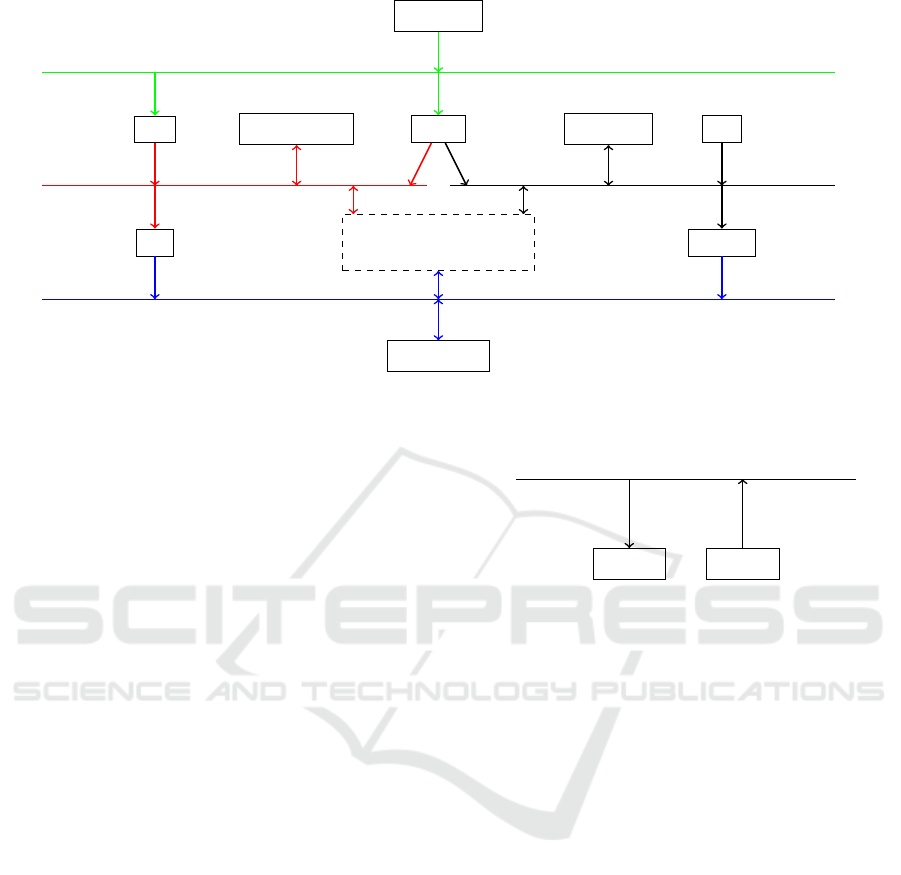
uncontrollable plants
gas
heat
electricity
cold
Figure 1: Example of a cell with four different grids (gas, heat, cold, electricity), ten different controllable and uncontrollable
plants and 17 connections between them.The abbreviations mean: HB = heating boiler, CHP = combined heat and power unit,
PV = photovoltaic system, AC = absorption chiller, RACM = refrigeration and air conditioning machine.
plants, all networks and the existing links between
them in a energy system. An important aspect is that
the flexibility definition remains the same even if a
cell is integrated into a higher-level cell. To achieve
this, flexibility is first of all considered at the lowest
level, i.e. at the plant level. If the flexibility of an
entire cell is defined as the aggregated flexibilities of
the individual plants contained in it, then if it is em-
bedded in a higher-level cell, only an extension of the
number of all considered plants is carried out. For a
single plant, on the one hand flexibility can describe
the possibility to vary a load (in form of purchased
or provided power) at a specific point of time or over
a time interval. A second type of flexibility is offe-
red when there is the possibility of load shifting over
time. That means a predefined load is deferrable or
even interruptible. Overall there can be flexibilities in
energy-related or temporal terms. Furthermore, only
such plants can offer flexibilities which can be con-
trolled in the described sense. Therefore the follo-
wing distinction between controllable and uncontrol-
lable plants is made in the discussed model:
(1) A plant can be controlled (called controllable) if
its power consumption or output can be control-
led/defined within a range permitted for the plant.
Limits of the permissible range can depend on
stochastic influencing variables. Such plants ful-
fill the requirements introduced in section 3.2.1 to
3.2.10.
(2) All plants that cannot be controlled are called un-
controllable. The power flows for these plants are
random variables for all time intervals.
plant 1 plant 2
network
consumption − + generation
Figure 2: Visualisation of two plants in a cell with different
flow direction and corresponding signs (+ indicates genera-
tion; - indicates consumption).
Another aspect that has to be taken into account
defining flexibility, is the interaction of different net-
works that supply power to the plants or into which
power is fed. Various energy vectors, such as electri-
city, gas, heat and cold, play a particularly important
role here. In this respect, the sign of the power should
indicate the direction in which it flows. Figure 2 il-
lustrates the flow directions with the corresponding
signs. If a plant consumes power from the grid, the
sign is negative and vice versa. An example of a cell
with different networks and plants is given in Figure
1.
3.2 Mathematical Model
The time interval for which all energy flows of a cell
are considered is indicated with [0, T] for T ∈ N where
T is the number of time steps. The variable t describes
a specific point in time within the interval [0, T]. The
time steps are discrete and in 15-minutes intervals to
draw a link to the scenario of peak demand manage-
ment. For other use cases the length of the time steps
can easily be modified. Some of our later constraints
have to be changed to these modifications.
Flexibility Definition for Smart Grid Cells in a Decentralized Energy System
133

Figure 3: Schematic illustration of the flexibility of two plants A
1
and A
2
with possible power flows P
1
and P
2
. Dependencies
to other plants of the cell were neglected for the sake of representability. The combinations of P
1
and P
2
in the gray area are
possible loads and the whole area reflects the total flexibility of the two plants at the time points t
1
and t
2
.
The number of plants in the cell under conside-
ration is given by Z and the plants are induced by
i ∈ {1, . . . , Z}
The differentiation of plants in controllable and non-
controllable is made using the parameter s ∈ {c, nc}.
The parameter n specifies the network from which
a plant draws power or into which a plant
feeds power. This implies that energy flows
take place exclusively between plants and net-
works i.e. any energy loss in networks is neg-
lected. The set of considered networks is given by
N = {E
1
, . .. , E
k
, H
1
, . .. , H
l
,C
1
, . .. ,C
m
, G
1
, . .. , G
o
},
where electricity grids are marked by E
j
1
, heat grids
by H
j
2
, cold grids by C
j
3
and gas grids by G
j
4
for
j
1
∈ {1, . . . , k}, j
2
∈ {1, . . . , l}, j
3
∈ {1, . . . , m} and
j
4
∈ {1, .. . , o}.
The variable P
t,i,s,n
describes the power consumed or
provided by plant i at time t. The network in which
the power transfer takes place is specified by the pa-
rameter n and the controllability of the plant by pa-
rameter s. Every P
t,i,s,n
is understood as the average
load within the time step [t,t + 1). Because not all
combinations of i, s and n exist just the real existing
links between networks and plants and the correspon-
ding indices are taken into account. The set of all
links between plants and networks can be described
as P = {(i, n)| the link between i and n exists}. The
number of these links is denoted by p = |P |.
For plants that cannot be controlled, their power flows
P
t,i,nc,n
represent stochastic quantities at all points t in
time. For the following theory it is assumed that fore-
casts on the time interval [0, T ] in the form of defined
values from R exist for all these uncontrollable power
flows.
In order to describe the flexibility of each plant
at a time t, conditions are placed on P
t,i,s,n
. The
set of all permissible values for P
t,i,s,n
forms the
flexibility of plant i at time t and is a subset of
R. It must be born in mind that the flexibility of a
single plant cannot be considered separately from the
behaviour/performance of other plants, since there
are dependencies between the consumed/disposed
powers of all plants. In addition, dependencies
between plants not only refer to a fixed point in
time, but also have to be taken into account across
time periods. The flexibility F , i.e. the set of all
permissible load profiles for an energy system (also
called cell), is therefore defined as follows:
Definition (Flexibility) Let E be an energy system
that includes Z plants and N networks and is consi-
dered on the discrete time interval [0, T ]. In addition,
the number of connections between plants and net-
works is indicated by p, where p ≤ Z ∗ N. Then the
flexibility F
E
of the energy system is given by the fol-
lowing subset of R
p∗T
:
F
E
=

x ∈ R
p∗T
| 3.2.1 to 3.2.10 applied

(1)
The entries of vector x represent the power flows be-
tween plants and networks at all times t ∈ [0, T ] and
therefore define a complete permissible load profile of
the following form:
x = (. . . , P
0,i,s,n
, . . . , P
T −1,i,s,n
, . . .) ∀(i, n) ∈ P
An active formulation of the conditions 3.2.1 to
3.2.10 only takes place for controllable plants. Power
flows of uncontrollable plants in the form of fixed, pre-
dicted values are taken into account indirectly (con-
sidering dependencies or conservation principles) if
necessary.
The flexibility concept defined in this way is visu-
alized in Figure 3 using the example of two (control-
lable) plants A
1
and A
2
with one network connection
each (P
1
and P
2
). In sections 3.2.1 to 3.2.10, the con-
ditions for x ∈ R
p∗T
are now discussed.
SMARTGREENS 2018 - 7th International Conference on Smart Cities and Green ICT Systems
134

3.2.1 Energy Conservation Principle for
Networks
In each network belonging to the cell, the sum of con-
sumption (negative sign) and generation/feed-in (po-
sitiv sign) must result in zero. Mathematically, this
can be described by the following equation:
∀n ∈ N ∀t ∈ [0, T ]
∑
i∈Z
P
t,i,s,n
= 0. (2)
The sum also includes the power flows of uncontrolla-
ble plants in form of fixed, previously forecast values.
3.2.2 Physical Limit Constraints
The power consumption or supply of each plant i is
subject to plant- and grid-inherent physical restricti-
ons in form of lower and upper bounds (LB and UB).
This is formulated as follows:
∀i, n ∃LB
1
, . . . , LB
p
,UB
1
, . . . ,UB
p
with p ∈ N, such that
LB
j
(i, n) ≤ P
t,i,c,n
≤ U B
j
(i, n) (3)
with
j ∈ {1, . . . , p}.
Power plants have often the physical limit constraints
LB
j
(i, n) = 0 and consuming plants U B
j
(i, n) = 0.
3.2.3 Specified Power at Specified Times
It is often the case that power consumption or sup-
ply of a plant i is prescribed for certain time intervals
[t, t +1). Therefore, at these points conditions are pro-
vided to P
t,i,c,n
in the following form:
P
t,i,c,n
= C(t, i, n). (4)
3.2.4 Dependencies Over Time
For some plants the provided or purchased power at
time t depends on the power of earlier points in time
˜
t with
˜
t ∈ [0, t). This can be modelled by setting up-
per and lower limits to the power that do not only de-
pend on i and n (physical limit constraints) but also on
P
˜
t,i,c,n
. If the power of plant i at time t to network n
depends on
˜
t
1
, . . . ,
˜
t
j
, the following condition is obtai-
ned:
LB = LB(i, n, P
˜
t
1
,i,c,n
, . . . , P
˜
t
j
,i,c,n
)
and
UB = UB(i, n, P
˜
t
1
,i,c,n
, . . . , P
˜
t
j
,i,c,n
)
with
LB ≤ P
t,i,c,n
≤ U B. (5)
3.2.5 Dependencies Between Plants
Just as the power of a plant i at time t can depend on
previous performances of the same plant, dependen-
cies between different plants are also possible. For
example, if the provided or purchased power of plant
i at time t to network n depends on the power of plant
h ∈ {1, . . . , Z} at times
˜
t
1
, . . . ,
˜
t
j
∈ [0,t], this can be
formulated as follows using upper or lower limit con-
straints:
LB = LB(i, n, P
˜
t
1
,h,s,n
, . . . , P
˜
t
j
,h,s,n
)
and
UB = UB(i, n, P
˜
t
1
,h,s,n
, . . . , P
˜
t
j
,h,s,n
)
with
LB ≤ P
t,i,c,n
≤ U B. (6)
3.2.6 Dependencies on Stochastic Environmental
Influences
In some cases, the upper and lower limits of the per-
missible power spectrum of a plant i at time t to net-
work n may also depend on environmental influences
EI
t
such as the global horizontal irradiance GHI
t
(in
the case of PV plants). Assuming that forecasts for
the time interval [0, T ] are available for such stochas-
tic influencing variables, the following dependencies
and restrictions on the power at time t result:
LB = LB(i, n, EI
t
)
and
UB = UB(i, n, EI
t
)
with
LB ≤ P
t,i,c,n
≤ U B. (7)
3.2.7 Number of Total Operation Hours
For some plants the operation hours are limited to a
certain number #S. This condition is modelled using
the indicator function 1:
∑
t∈[0,T ]
1
{|P
t,i,c,n
|>0}
!
: 4 ≤ #S (8)
The number of time intervals having positive or
negative power is divided by 4 in order to take into
account that the time steps are set at quarter-hourly
basis.
Flexibility Definition for Smart Grid Cells in a Decentralized Energy System
135

3.2.8 Specified Energy at Specified Times
Often, such as in the case of batteries, a storage de-
vice must hold a certain amount of energy C. If the
condition should be fulfilled at time t
1
, this can be
guaranteed by the following inequality:
∑
t∈[0,t
1
]
P
t,i,c,n
·
1
4
h ≥ C(0, t
1
, i) (9)
3.2.9 Specific Switch-on and Switch-off Times
There are plants that can only be switched on or off
for a limited number of consecutive time intervals.
A classic example is a ventilation system that can-
not be switched off for longer than a certain period of
time. On the other hand, there are systems that must
be switched on/off for a minimum number of conse-
cutive time intervals. Another variant is a plant that
hast to comply with a predefined switch-on/switch-
off pattern. Such a pattern could be the condition that
after switching off the ventilation for two time units,
it must be switched on for the same period of time.
Some of the most frequently required conditions are
formulated below.
For this purpose, the binary variable δ
t,i
is defined by
δ
t,i
=
(
0 , if plant i is switched off at time t
1 , if plant i is switched on at time t
1. The plant is allowed to be switched on for a max-
imum of k consecutive time steps. To ensure this
condition, the inequality
t+k
∑
˜
t=t+1
δ
˜
t,i
− (k − 1) ≤ 1 − δ
t,i
must be fulfilled for all t ∈ {0, . . . , T − k}.
2. The plant must be switched on for at least k con-
secutive time steps. This condition is met if
t+k
∑
˜
t=t+2
δ
˜
t,i
−(k −1) ≥ (1−k)(1−δ
t+1,i
)+(1−k)δ
t,i
and applies for all t ∈ {0, . . . , T − k}.
3. The plant may be switched off for a maximum of k
consecutive time steps. That means the inequality
t+k
∑
˜
t=t+1
δ
˜
t,i
− 1 ≥ −δ
t,i
has to be valid for all t ∈ {0, . . . , T − k}.
4. The plant must be switched off for at least k con-
secutive time steps. This condition holds if
t+k
∑
˜
t=t+2
δ
˜
t,i
≤ (k − 1)δ
t+1,i
+ (k − 1)(1 − δ
t,i
)
for all t ∈ {0, . . . , T − k}.
5. If the plant has been switched of for k consecutive
time steps, then it must be switched on for l con-
secutive time steps. To ensure this condition, the
inequality
t+k+l−1
∑
˜
t=t+k
δ
˜
t,i
− l ≥ −l ·
t+k−1
∑
˜
t=t
δ
˜
t,i
must be fulfilled for all t ∈ {0, . . . , T − k − l + 1}.
3.2.10 Energy Conservation Principle for Plants
When a plant interacts with different networks like
gas, electricity, heat and cold grids, it must be en-
sured that the energy conservation principle is fulfil-
led. A co-generation plant, which draws power from
the gas grid and supplies power to the electricity and
heat grid, is a good example. Let {n
i
0
, . . . , n
i
k
} desig-
nate the different networks from which a plant i draws
power at time t and {n
i
k+1
, . . . , n
i
l
} the different net-
works fed by plant i. When η describes the efficiency
of plant i, then the following equation must apply for
all t ∈ [0, T ]:
−η
n
i
k
∑
j=n
i
0
P
t,i,s, j
=
n
i
l
∑
j=n
i
k+1
P
t,i,s, j
(10)
The powers provided to different networks are in
a certain ratio to each other, which is why
−η
n
i
k
∑
j=n
i
0
P
t,i,s, j
=
1
x
j
P
t,i,s,n
j
(11)
must also be fulfilled for all j ∈ {k + 1, . . . , l} and
∑
j
x
j
= 1. The x
j
result from the partial efficiencies
η
k+1
, . . . , η
l
through
x
j
=
η
j
η
∀ j ∈ {k + 1, . . . , l}.
4 EVALUATION
Since the definition given in this paper is first of all
theoretical in nature and will be incorporated into op-
timization problems for load profiles of cells in a next
step, an evaluation at this point in time will also take
place on a theoretical level.
SMARTGREENS 2018 - 7th International Conference on Smart Cities and Green ICT Systems
136

One aspect to be considered is the possibility that con-
ditions 3.2.1 through 3.2.10 in their current formula-
tion may approximate reality too simplistic in some
cases. This is explained by the fact that a compromise
must be found between a complete representation of
reality and an excessively high complexity of the so-
lution space (in the form of flexibility). The extent to
which the degree of abstraction chosen in this paper
proves suitable for the application remains to be ve-
rified. However, since a generic approach to describe
flexibility was the main objective of this work, there
only has been a deliberate simplification for condi-
tion 3.2.10. The complexity was reduced by assuming
the efficiency η to be independent of the power flows.
Actually, the following should apply, with the notati-
ons from 3.2.10:
η = η(P
t,i,s,n
i
0
, . . . , P
t,i,s,n
i
k
) (12)
The same applies to the proportion of power pro-
vided to power consumed by the plant, which also
changes depending on the latter:
x
j
= x
j
(P
t,i,s,n
i
0
, . . . , P
t,i,s,n
i
k
) (13)
for all j ∈ {k + 1, . . . , l} and
∑
j
x
j
= 1.
The example of a cell from Figure 1 will be used to
evaluate, whether the conditions formulated in 3.2.1
to 3.2.10 are suitable to describe the flexibility pre-
sent in this cell.
First of all, it is determined that the observation pe-
riod should be one day which equals 96 time steps.
The number of plants Z is given by 10 and the num-
ber of networks by 4 (gas, heat, electricity and cold),
with a total of p = 17 connections between plants and
networks. The flexibility can then be formulated ac-
cording to definition (1) as follows:
F
E
=
n
x ∈ R
17∗96
| 3.2.1 to 3.2.10 apply
o
In practice, the set of all possible load profiles is first
of all limited by the fact that the power balance within
a network must always be zero. In the case of Figure
1, the equation in 3.2.1 must therefore apply specifi-
cally to the four grids gas, heat, electricity and cold
(described as the set N = {G, H, E,C}):
∀t ∈ [0, 96 − 1]
10
∑
i=1
P
t,i,s,n
= 0.
Secondly, technical/physical restrictions of plants and
also networks for determining cell flexibility must be
taken into account. If, for example, the CHP, the HB,
or the AC is considered, plausible physical limit con-
straints could be the following:
CHP: Combustion heat output 0 kW or between
500 kW and 2 MW. Electrical power 0 kW or be-
tween 500 and 2 kW.
HB: Combustion heat output 0 kW or between 500
kW and 4, 9 MW.
AC: Cooling capacity 0 kW or between 50 kW and
200 kW.
If these restrictions are combined, exactly the upper
and lower bounds defined in 3.2.2 are obtained.
Further constraints arise as a result of temporal de-
pendencies in the power flows, as in this example for
the two storages (heat and ice storage). The general
formulation in 3.2.4 results into
0 ≤
t
∑
˜
t=0
(P
˜
t,HS,c,H
·
1
4
h) ≤ S
max
∀t ∈ [0, 96 − 1]
⇔ −
t−1
∑
˜
t=0
P
˜
t,HS,c,H
≤ P
t,HS,s,H
≤ S
max
·
4
h
−
t−1
∑
˜
t=0
P
˜
t,HS,c,H
where the two terms on the left and right side repre-
sent the lower and upper bounds respectively and S
max
is the maximal storage capacity of the heat storage. In
the case of the ice storage, LB and UB can be formu-
lated in the same way.
For the PV system of the cell, the upper power limit
also depends on the stochastic influencing variable of
the global horizontal irradiance. As from 3.2.6
UB = UB(PV, E, GHI
t
) = f (GHI
t
)
is another condition for the set of all permissible load
profiles, where the function f determines the relati-
onship between the predicted value of GHI
t
and the
maximum possible power generation.
Next, the maximum switch-off time prescribed for the
RACM must be taken into account. If the air qua-
lity is not to deteriorate too much, a plausible speci-
fication could be half an hour. Using the binary va-
riable δ
t,i
, defined in 3.2.9, and k = 2 (2 · 15min =
30min), the following constraint is obtained for all
t ∈ {0, . . . , (96 − 1) − 2}:
t+2
∑
˜
t=t+1
δ
˜
t,RACM
− 1 ≥ −δ
t,RACM
Finally, in order to describe the flexibility in the ex-
emplary energy system shown in Figure 1, it should
be noted that the energy balance for individual plants
connected to more than one network will be maintai-
ned. In this context it concerns the four plants HB,
AC, CHP and RACM, whereby in the following the
condition from 3.2.10 is formulated as an example for
the CHP. It is assumed that the CHP has an electri-
cal efficiency of 43, 5% and a thermal efficiency of
41, 5%, resulting in an overall efficiency of 85%. The
Flexibility Definition for Smart Grid Cells in a Decentralized Energy System
137

following equations must therefore be fulfilled for all
t ∈ [0, 96 − 1]:
−0.85 · P
t,CHP,c,G
= P
t,CHP,c,H
+ P
t,CHP,c,E
and
−0.85 · P
t,CHP,c,G
=
0.85
0.435
· P
t,CHP,c,E
and
−0.85 · P
t,CHP,c,G
=
0.85
0.415
· P
t,CHP,c,H
This example shows that the generic description of
flexibility made in this paper is suitable for applying
it to a wide range of cells.
5 CONCLUSION AND OUTLOOK
In order to create a common communication basis
for cells of different types enabling the exchange of
information regarding existing and thus usable flexi-
bility, a generic definition of flexibility is developed
in this paper. This is particularly important against
the background of the energy transition, since the
use of flexibility within a cellularly structured energy
system is one of the most widely pursued approaches
to deal with the challenges of an increasingly decen-
tralised energy system.
The basic idea is to define flexibility within cells
containing any number of plants and networks as
the set of all possible and permissible load profiles.
This can be described as a subset of R
p·T
, where
p describes the number of all existing connections
between plants and networks and T the number of
considered time steps. Each point defines a complete
load profile for all networks and all plants for a
pre-defined, future time interval. In order to deter-
mine the subset, conditions have been introduced
which include interdependencies between plants and
laws for energy conservation within networks and
individual plants. Further criteria for the definition of
flexibility are that it creates a suitable solution space
for load optimization problems within cells, enables
easy integration into higher-level cells and supports
the modelling of power flows at plant level.
Individual sub aspects in the plant behaviour, such
as start-up ramps, energy loss in networks or power-
dependent efficiency ratios, are currently still being
neglected, as these would not change the basic idea
of describing the system, but would create additional
complexity. However, such aspects can be added to
the given definition at any time.
Based on the now generally defined concept of
flexibility, it is to be investigated how it can be embed-
ded in different methods for the optimization of load
profiles within but also across cells. This also raises
the question of the visualization ability of flexibility,
which is currently still implicitly described by boun-
dary conditions to the permissible subset of R
p·T
.
Therefore, this aspect is also closely related to the in-
vestigation of possibilities for an explicit representa-
tion of flexibility. It may be necessary to make further
simplifying assumptions on the energy systems under
consideration in order to facilitate the application of
the definition within the context of load optimization
in real cells.
In addition, another application objective of the flexi-
bility definition given in this paper is to be seen in the
context of fleet management of electric vehicles. The
energy management system of a shared electric vehi-
cle fleet described in (Ostermann and Koetter, 2016)
implements the flexibility idea presented in this paper
for a special case in practice. This offers a possible
application case in which a transfer of the theoreti-
cal definition into practice can be the subject of future
research work.
ACKNOWLEDGEMENTS
The work published in this article was funded by
the Bundesministerium f
¨
ur Wirtschaft und Energie
(BMWi) under the project C/sells under the promo-
tional reference 03SIN125.
REFERENCES
Allerding, F., Mauser, I., and Schmeck, H. (2014). Customi-
zable Energy Management in Smart Buildings Using
Evolutionary Algorithms, pages 153–164. Springer
Berlin Heidelberg, Berlin, Heidelberg.
Gellings, C. W. (1985). The concept of demand-side mana-
gement for electric utilities. Proceedings of the IEEE,
73(10):1468–1470.
Gottwald, S., Ketter, W., Block, C., Collins, J., and Wein-
hardt, C. (2011). Demand side management - a si-
mulation of household behavior under variable prices.
Energy Policy, 39(12):8163–8174.
Greer, C., Wollman, D., Prochaska, D., Boynton, P., Mazer,
J., Nguyen, C., FritzPatrick, G., Nelson, T., Koepke,
G., and Jr, A. H. (2014). Nist framework and road-
map for smart grid interoperability standards. Techni-
cal Report 3.0, US National Institute of Standards and
Technology.
Khoury, J., Mbayed, R., Salloum, G., and Monmasson,
E. (2016). Predictive demand side management of
a residential house under intermittent primary energy
SMARTGREENS 2018 - 7th International Conference on Smart Cities and Green ICT Systems
138

source conditions. Energy and Buildings, 112:110 –
120.
Liu, Y., Yuen, C., Hassan, N. U., Huang, S., Yu, R., and Xie,
S. (2014). Electricity cost minimization for a micro-
grid with distributed energy resource under different
information availability. IEEE Transactions on Indus-
trial Electronics, 62:2571–2583.
Liu, Y., Yuen, C., Yu, R., Zhang, Y., and Xie, S. (2015).
Queuing-based energy consumption management for
heterogeneous residential demands in smart grid.
IEEE Transactions on Smart Grid, 7:1650–1659.
Mauser, I. (2017). Multi-modal Building Energy Manage-
ment. PhD thesis, Karlsruher Institut f
¨
ur Technologie
(KIT).
Mauser, I., M
¨
uller, J., Allerding, F., and Schmeck, H.
(2016). Adaptive building energy management with
multiple commodities and flexible evolutionary opti-
mization. Renewable Energy, 87:911–921.
Ostermann, J. and Koetter, F. (2016). Energy-management-
as-a-service: Mobility aware energy management for
a shared electric vehicle fleet. In Proceedings of
the 5th International Conference on Smart Cities and
Green ICT Systems - Volume 1: SMARTGREENS,, pa-
ges 340–350. INSTICC, SciTePress.
Palensky, P. and Dietrich, D. (2011). Demand side manage-
ment: Demand response, intelligent energy systems,
and smart loads. IEEE Trans. Ind. Inf., 7(3):381–388.
Smart Grid Coordination Group (2014). Sg-cg/m490/l flex-
ibility management - overview of the main concepts
of flexibility management. CEN-CENELEC-ETSI
Smart Grid Coordination Group.
Smart Grids-Plattform Baden-W
¨
urttemberg e.V (2017).
Official c/sells website. http://www.csells.net/de/.
Accessed: 2017-12-21.
Tushar, W., Chai, B., Yuen, C., Smith, D. B., Wood,
K. L., Yang, Z., and Poor, H. V. (2014). Three-party
energy management with distributed energy resources
in smart grid. IEEE Transactions on Industrial Elec-
tronics, 62:2487–2498.
Weckmann, S., Kuhlmann, T., and Sauer, A. (2017). Decen-
tral energy control in a flexible production to balance
energy supply and demand. Procedia CIRP, 61(Sup-
plement C):428 – 433. The 24th CIRP Conference on
Life Cycle Engineering.
Flexibility Definition for Smart Grid Cells in a Decentralized Energy System
139