Demand Response of Medical Freezers in a Business Park Microgrid
Rosa Morales Gonz
´
alez
1
, Madeleine Gibescu
1
, Sjef Cobben
1,2
,
Martijn Bongaerts
2
, Marcel de Nes-Koedam
2
and Wouter Vermeiden
2
1
Electrical Energy Systems Group, Department of Electrical Engineering, Eindhoven University of Technology,
5612AP Eindhoven, The Netherlands
2
Alliander N.V., 6812AH Arnhem, The Netherlands
Keywords:
Demand Response, Genetic Algorithm, Local RES Integration, Physical System Modeling, Smart Grid.
Abstract:
This paper presents a demand response (DR) framework that utilizes the flexibility inherent to the thermo-
dynamic behavior of four groups of independently-controlled medical freezers in a privately-owned business
park microgrid that contains rooftop photovoltaics (PV). The optimization objectives may be chosen from the
following 3 options: minimizing electricity exchanges with the public grid; minimizing costs by considering
prices and RES availability; and minimizing peak load. The proposed DR framework combines thermody-
namic models with automated, genetic-algorithm-based optimization, resulting in demonstrable benefits in
terms of cost, energy efficiency, and peak power reduction for the consumer, local energy producer, and grid
operator. The resulting optimal DR schedules of the freezers are compared against unoptimized, business-as-
usual scenarios with- and without PV. Results show that flexibility can be harnessed from the thermal mass of
the freezers and their contents, improving the cost- and energy performance of the system with respect to the
business-as-usual scenarios.
1 INTRODUCTION
Increasing distributed generation from renewable
energy sources (DG-RES), such as solar and wind,
into electricity networks poses several challenges due
to the resources’ stochastic nature (Hewicker et al.,
2012). This variability brings about a loss of flexi-
bility in the generation side of the power system va-
lue chain, since the electricity generation profile can
no longer ramp up or down to adapt to the load pro-
file. Within the evolution of power systems, the con-
cept of smart grids proposes different technical solu-
tions that can harness flexibility from other sources
to compensate for the loss of flexibility from the ge-
neration side: e.g., enhanced monitoring and control
functionalities, electrical and/or thermal storage, no-
vel electricity market designs, and increased demand-
side flexibility through demand response (DR) pro-
grams (Huber et al., 2014; Alizadeh et al., 2016). De-
mand response is defined as the set of “actions vo-
luntarily taken by consumers [and/or prosumers] to
change their energy usage —either in terms of quan-
tity or timing— in response to an external control sig-
nal” (Morales Gonz
´
alez et al., 2016), e.g., price or a
direct command from the aggregator or system opera-
tor.
Thermostatically-controlled loads have become a
valuable flexible resource of DR programs in the resi-
dential sector, where water heaters (Gela
ˇ
zanskas and
Gamage, 2016), refrigerators (Liu et al., 2014), and
HVAC systems (Yoon et al., 2014) have been targe-
ted for the implementation of DR programs in the
residential sector. However, in order to unlock their
full potential, the (small) loads have to be aggregated
in large numbers. This is not always possible in pi-
lot programs involving residential consumers, due to
low participation of the customer base, limited resour-
ces and large investment requirements, as discussed in
(He et al., 2013; Klaassen et al., 2014; D’hulst et al.,
2015; Labeeuw et al., 2015).
Commercial and industrial (C&I) consumers, on
the other hand, have an overall higher consumption
footprint and a higher peak demand (European En-
vironment Agency, 2017). Furthermore, C&I consu-
mers are usually located in concentrated areas such
as business/industrial parks, which facilitates aggre-
gation and makes this type of end-users interesting for
applying DR programs (Ashok and Banerjee, 2000;
Gr
¨
unewald and Torriti, 2013). Several strategies have
been proposed for different types of heavy industry
120
Morales González, R., Gibescu, M., Cobben, S., Bongaerts, M., de Nes-Koedam, M. and Vermeiden, W.
Demand Response of Medical Freezers in a Business Park Microgrid.
DOI: 10.5220/0006801001200129
In Proceedings of the 7th International Conference on Smart Cities and Green ICT Systems (SMARTGREENS 2018), pages 120-129
ISBN: 978-989-758-292-9
Copyright
c
 2019 by SCITEPRESS – Science and Technology Publications, Lda. All rights reserved

in works such as (Matthews and Craig, 2013; Mitra
et al., 2013; Finn and Fitzpatrick, 2014), but DR is
still not implemented systematically in this sector be-
cause industrial consumers’ energy needs vary gre-
atly from one another and applications for DR can be
restricted in scope due to the nature or sensitivity to
changes of the processes inherent to the industry (Sa-
mad and Kiliccote, 2012; Ton and Smith, 2012).
Authors such as the ones from (Zavala, 2013; Ma
et al., 2015; Yin et al., 2016; Hurtado et al., 2017)
have written extensively on the flexibility of commer-
cial buildings in cities through buildings’ passive ther-
mal capacitance and HVAC controls. Their findings
on the DR potential of commercial buildings are es-
pecially relevant to the case of the Netherlands, where
the service industry is the second largest energy con-
sumer behind heavy industry (Centraal Bureau voor
de Statistiek, 2017a). This sector has seen steady
and rapid growth in the past twenty years and contri-
butes to the highest added value and employment in
the Dutch economy (Compendium voor de Leefom-
geving, 2017).
In this work, we focus on the DR potential of the
health services sector, ranked in the top three sectors
of the Dutch economy (Centraal Bureau voor de Sta-
tistiek, 2017b). We propose and test a DR framework
with a case study of a business park microgrid with
local PV generation in which the flexible load is a me-
dical freezing warehouse. Freezer loads are shifted in
time by automated DR actions, controlling the medi-
cal freezers in four independent clusters, while trea-
ting PV production as a curtailable/reparameterizable
resource. The case study evaluates the benefits of the
DR program over a 48-hour time window with a reso-
lution of 15-minutes. We study a 48-hour optimiza-
tion window in order to observe the temperature dyn-
amics of the freezers on a longer term than day-ahead,
and to solve a more complex problem that can test the
robustness of our framework.
Our main contributions are the iterative embed-
ding of the thermodynamic freezer model into an op-
timization algorithm to form a single DR framework,
and its application to a real-world situation. This
work explores 1) how flexibility can be harnessed
from the freezer contents’ thermal mass, and 2) what
the resulting benefits are in terms of cost, energy effi-
ciency and peak load reduction for the consumer, the
local DG-RES producer, and the operator of the busi-
ness park microgrid.
The rest of the paper is organized as follows:
Section 2 describes the mathematical models, and
Section 3 describes the case study used for this work.
In Sections 4 and 5, results are presented and dis-
cussed. Finally, conclusions and directions for future
Freezer Enclosure
Indoor environment
Ambient
R
ic-in
R
e,1,1
R
e,1,2
R
e,1,3
R
e,1,4
R
e,2,1
R
e,2,2
R
e,2,3
R
e,2,4
R
e,n,1
R
e,n,2
R
e,n,3
R
e,n,4
R
in-sup
Q˙
sup
T
amb
T
in
T
sup
T
ic
(mc
p
)
ic
(mc
p
)
e,2
(mc
p
)
e,n
(mc
p
)
e,1
(mc
p
)
in
Figure 1: Equivalent RC circuit of the medical freezers.
work are stated in Section 6.
2 METHODOLOGY
This section describes the mathematical models and
algorithms that make up the physical models, in com-
bination with our optimization-based DR framework.
2.1 Thermodynamic Modeling
The thermodynamics of the medical freezers in the
research facility can be described by a first-order dy-
namic system, as described in works such as (Za-
paroli and de Lemos, 1996; Lampropoulos et al.,
2013; Kalsi et al., 2011; Hurtado et al., 2015; Wil-
son et al., 2015). The generic, lumped parameter
resistance/capacitance (RC) circuit model, shown in
Figure 1, is used to achieve a better understanding
of how the thermal mass of buildings can unlock
demand-side flexibility in terms of available shifting
power and duration and possible energy/cost savings.
This simplified representation of end-user premises
allows us to 1) capture first-order transients without
having to perform a heavily-detailed simulation, and
2) facilitate the real-time implementation of the opti-
mization framework we use in our DR program. The
system of equations describing the thermodynamic
behavior of the medical freezers is given in equation
(1):
(mc
p
)
ic
dT
ic
(t)/dt = −(T
ic
− T
in
)/R
ic−in
(1a)
(mc
p
)
in
dT
in
(t)
dt
=
T
ic
− T
in
R
ic−in
−
T
in
− T
sup
R
in−sup
−
N
∑
n=1
T
in
− T
e,n
R
e,n,1
+ R
e,n,2
(1b)
(mc
p
)
e,n
dT
e,n
(t)
dt
=
T
in
− T
e,n
R
e,n,1
+ R
e,n,2
−
T
e,n
− T
amb
R
e,n,3
+ R
e,n,4
∀n ∈ [1,N]
(1c)
0 = (T
in
− T
sup
)/R
conv
+
˙
Q
sup
(1d)
Demand Response of Medical Freezers in a Business Park Microgrid
121

where (mc
p
)
x
denotes heat capacity in J/K; dT
x
(t)/dt,
is the rate of change temperature with respect to time
in K/s; and R
x
denotes thermal resistance in K/W. The
subscript x is a stand-in for the subscripts ic, in, sup
and e,n, (see corresponding blocks in Figure 1) which
denote the freezer’s interior contents, indoor air, heat
supply system (evaporator coil), and n number of en-
closure elements out of a total N (e.g., freezer roof,
walls, floor), respectively. T
amb
is the ambient tem-
perature (i.e. temperature of the conditioned space in
which the freezers are kept) as a function of time in
degrees Kelvin (K),
˙
Q
sup
is the heat extracted by the
freezer’s mechanical cooling system in watts, and T
sup
is the supply temperature of the mechanical cooling
system in K.
Mechanical heat extracted is related to electrical
power consumption,
˙
W
el
, through the coefficient of
performance (COP) of the freezers’ mechanical cool-
ing system, defined by (2):
COP =
˙
Q
sup
/
˙
W
el
(2)
Assuming that the conditioned space in which the
freezers are kept is maintained at a constant tempera-
ture to ensure the optimal operation of the mechanical
refrigeration system, we may assume a constant COP;
hence, mechanical heat extracted is given by (3):
˙
Q
sup
= COP ×
˙
W
el
(3)
Finally, assuming we can independently control
the operation of the medical freezer in i clusters, the
electricity consumption of each cluster at time t is gi-
ven by (4):
E(i,t) =
Z
t
t−1
˙
W
el
(i,t)dt
(4)
2.2 Optimization Problem Formulation
Let us consider that the ON/OFF signal of the medical
freezers of cluster i at time t is defined by the binary
variable β(i,t). The net energy imported from the
grid of all I freezers at the research facility, E
net
(t),
after combining the predicted contribution of local
DG-RES in the microgrid E
RES
(t) and the electricity
consumption of the independently-controlled freezer
clusters i at time t, E(i,t), is expressed by (5):
E
net
(t) =
I
∑
i=1
β(i,t)E(i,t) − E
RES
(t)
(5)
The optimization problem (6a) signifies choosing
the ON/OFF switching schedules (β(i,t)) and the PV
production schedule E
RES
(t) over the whole time ho-
rizon, with the objective of minimizing energy ex-
changes with the regional grid (7), peak power con-
sumption (8), or overall energy cost (12). Each of
these optimization problems is analyzed separately.
The freezer temperatures (T
in
(i,t)) must not exceed
the critical values required by the end-users (6b). Phy-
sical constraints of local DG-RES production (6c) are
considered. Finally, the rated capacity of the con-
nection, P
max
, should not be exceeded (6d). The opti-
mization problem takes on the form (6):
min
β,E
RES
Ω = Φ (6a)
s.t. T
min
(i,t) ≤ T
in
(i,t) ≤ T
max
(i,t) ∀i,t (6b)
0 ≤ E
RES
(t) ≤ E
max
RES
(t) ∀t (6c)
|P
net
| ≤ P
max
(6d)
with P
net
(t) =
∑
I
i=1
β(i,t)
˙
W
el
(i,t) −P
RES
(t). Φ stands
in for Φ
e
(7) in the energy consumption minimization-
, Φ
p
(8) in the peak load reduction- , and Φ
c
(12) in
the energy cost minimization problem variants:
Φ = Φ
e
=
T
∑
t=1
|E
net
(t)| (7)
Φ = Φ
p
= max(|P
net
|) (8)
For the cost optimization problem, let λ
RES
be
the price per kilowatt-hour the local consumer pays
for buying locally-produced energy in the microgrid,
λ
grid
the price for buying electricity from the regio-
nal electricity supplier, and λ
f eedin
the tariff the local
DG-RES producer gets for exporting PV to the regio-
nal distribution network. Let us assume that the DG-
RES producer sells its electricity at a lower price than
the consumer would pay for electricity from the regi-
onal electricity supplier, and that the feed-in tariff it
gets for feeding the electricity back into the regional
network is considerably less than that it receives for
selling electricity locally within the microgrid (9):
λ
f eedin
 λ
RES
(t) < λ
grid
(t) ∀t (9)
The total cost for the consumer is given by (10):
T
∑
t=1
(λ
RES
(t)E
RES
(t) + λ
grid
(t)E
imports
(t)) (10)
where E
RES
(t) is energy consumed from local DG-
RES, and E
imports
(t) is energy consumed from grid
imports in the microgrid —i.e., when E
net
> 0— at
time t. The total revenue for the DG-RES producer
from feeding in energy back into the grid —i.e., when
E
net
> 0— is denoted E
exports
(t) and defined as (11):
T
∑
t=1
(λ
RES
(t)E
RES
(t) + λ
f eedin
(t)E
exports
(t)) (11)
SMARTGREENS 2018 - 7th International Conference on Smart Cities and Green ICT Systems
122

Maximizing producer revenue and minimizing
consumer costs, we have:
Φ = Φ
c
=
T
∑
t=1
(λ
grid
(t)E
imports
(t)
− λ
f eedin
(t)E
exports
(t))
(12)
Constraint (6b) determines the flexibility of the
freezer and enforces the critical temperature ranges
for each freezer cluster i: T
min
(i,t) and T
max
(i,t). The
values of T
in
(i,t) are obtained from the thermodyna-
mic freezer submodels. Constraint (6c) enforces the
physical upper and lower bounds of local DG-RES
production. The resulting non-linear, mixed-integer
optimization problem is too complex to be solved by
traditional methods in reasonable time. From the fa-
mily of heuristic search techniques, we opted for the
genetic algorithm (GA) for its ability to efficiently
deal with both continuous and discrete decision va-
riables.
2.3 Interaction Between Models
While conventional freezer temperature controls have
a fixed set-point temperature and fixed temperature
trip points based on indoor air temperature measure-
ments, our multiphysics DR framework couples and
iteratively intertwines the thermodynamic freezer mo-
dels with the GA-based optimization framework to:
1) calculate temperature limits based on the freezer
contents instead of the indoor air to gain extra flexi-
bility from the products’ inherent thermal mass; and
2) to devise optimal on/off strategies for all freezer
clusters in the building, such that the objectives of
minimal cost, maximal energy self-sufficiency or mi-
nimum peak load are achieved. Note that the opti-
mization problem will determine the entire 48-hour
switching schedule in advance of real-time, assuming
perfect knowledge and/or accurate forecasts of all in-
fluencing factors: feed-in tarrifs, wholesale and local
market prices, and short-term PV production.
3 CASE STUDY
This section describes the case study for which the
simulation experiments were performed, as well as all
relevant technical characteristics.
Our DR framework is applied to a freezing ware-
house used for medical research in the Netherlands.
The medical freezing facility is located in a busi-
ness park that operates as a local, private microgrid
interconnected to the regional grid via a consumer
substation. Grid constraints are not an issue in this
case, since all network assets have been overdimensi-
oned. A 250-kWp photovoltaic installation consisting
of 1700 m
2
of crystalline PV panels is also coupled
to the business park microgrid through the consumer
substation. The PV modules are made of crystalline
silicone, and have a 15% efficiency. The energy con-
version efficiency of the PV modules is 80%. Overall,
the PV system efficiency is thus 12%. Electricity ge-
nerated locally by the PV installation is 157 MWh/y.
The medical freezing facility consumes approxima-
tely 1.4 GWh/y. It stores blood samples at a tempera-
ture of -80
◦
C in 120 freezer units. The freezer units
consume approximately 500 MWh/y in total, repre-
senting 35% of the total energy consumption in the
medical freezing facility.
The blood samples are preserved in a glycerol so-
lution for long-term storage. In setting our flexibility
thresholds for the freezer temperatures, we refer to in-
dustry best practices. These dictate that the tempera-
ture of the glycerolized red blood cells during storage
should not exceed -60
◦
C in order to avoid the de-
terioration of the samples (Maharashtra State Blood
Transfusion Council, 2014; Eftekhar, 1989; Wessling
and Blackshear, 1973). We set a conservative flexibi-
lity temperature upper limit of -70
◦
C to remain well
within the limits for sample quality preservation. The
temperature of the blood samples, (i.e., the tempera-
ture of the freezers’ internal contents, T
ic
in Figure 1
and eq. (1) will be used for the constraints formu-
lation of the optimization problem. This means that
T
ic
will be allowed to oscillate between -80 and -70
◦
C
with a tolerance of ±0.3
◦
C to account for system de-
lay in our GA-based controller.
The density and specific heat capacity of glycer-
olized red blood cells for the freezer working tempe-
ratures are compiled from (Eftekhar, 1989; Wessling
and Blackshear, 1973), and are shown in Table 1, and
compared against values for whole blood, as a refe-
rence. The values for glycerolized red blood cells will
be used in our DR framework’s building models to re-
present the internal contents of the medical freezers.
In this work, we assume that 1) the internal con-
tents of the freezer are already “at temperature”, and
2) there is no in- or outflow of samples during the 48h
time horizon of the DR optimization problem. In ot-
her words, the mechanical refrigeration system of the
freezers are only used to maintain the product tem-
perature. We contend this is a reasonable assumption
given that the medical freezing warehouse is a long-
term research facility in which samples are kept in
storage in the order of years, even decades.
In our energy calculations for the medical research
freezing facility, we neglect the base electricity load
Demand Response of Medical Freezers in a Business Park Microgrid
123

Table 1: Thermophysical properties of blood components.
Blood component ρ [kg/m
3
] c
p
[kJ/(kgK)]
Glycerolized red blood cells 1063 1.5
Whole blood 980 3.6
Time [h]
0 5 10 15 20 25 30 35 40 45
0
0.02
0.04
λ
grid
λ
RES
λ
feedin
Figure 2: Dynamic electricity prices for the end-users of the
microgrid.
and any loads triggered by human interaction. Hea-
ting or cooling loads required to balance ventilation
and internal heat gains/losses from lighting, people,
and equipment could be additional sources of flexibi-
lity in the building, but are not taken into considera-
tion in the present case study.
We assume that all end-users are subjected to the
same hourly electricity prices; and that electricity pri-
ces and PV generation for the optimization horizon
can be forecasted with a reasonable degree of accu-
racy. Expected day-ahead electricity prices
1
and PV
generation values for average irradiation days
2
used
in the simulations are shown in Figure 2 and Figure 3.
Three optimization objectives are considered se-
parately: 1) energy minimization (i.e., reducing
energy exchanges with the regional grid), 2) cost mi-
nimization, and 3) peak load minimization. The op-
timization results are compared against a Business-
As-Usual (BAU) scenario, where temperature con-
trol in the freezers is driven by their conventional,
continuously-operating thermostats with a fixed set-
point and deadband. We compare results of switching
all 120 freezers at the same time in the BAU scena-
rio (worst-case scenario for peak load) against having
four clusters of 30 freezers each that can be indepen-
dently controlled. Because grid constraints are not
an issue in the present case study, we set P
max
to the
1
Based on data from https://transparency.entsoe.eu/
2
Based on data from http://www.soda-pro.com/web-
services#radiation
Time [h]
0 5 10 15 20 25 30 35 40 45
Power [W]
× 10
4
0
5
10
15
Figure 3: PV production profiles for two consecutive
average solar irradiation days in the Netherlands (1700m
2
,
system efficiency 12%).
worst-case scenario for peak load, or 132 kW, in con-
straint (6d).
The design variables of the optimization problem
are the 15-minute switching schedules of the mecha-
nical refrigeration system for all freezer clusters, bi-
nary variable β(i,t), and the 15-minute DG-RES pro-
duction schedules, E
RES
(t). E
RES
is a continuous non-
negative variable on the interval [0,1] based on the
maximum forecasted production for that 48-hour time
horizon. For the 48-hour time window of the case
study, β has a length of 193 elements per i cluster
of freezers, and the microgrid-aggregated E
RES
has a
length of 193, resulting in a phenotype of 965 ele-
ments. Results were obtained by parallelizing the
GA computations into twenty-eight pools of workers
using MATLAB’s Parallel Computing Toolbox. The
simulations were carried out using an Intel Xeon CPU
with two processors running at 2.6 GHz.
3.1 Freezer Model
Each of the ultra-low temperature freezers used in the
medical research facility have a rated capacity of 1.1
kW and a COP of 0.575 at T
amb
= 25
◦
C. Their elec-
tricity consumption under no-load conditions —i.e.,
with an empty freezer— at a setpoint of -80
◦
C is 11.5
kWh/day. The peak load when all freezers are on at
the same time is 132 kW.
The freezers’ external and internal dimensions are
1030 × 882 × 1993 mm and 870 × 600 × 1400 mm,
respectively. The freezer enclosures are 80 mm-
thick, and consist of vacuum-insulated panels sand-
wiched between painted AISI type 304 stainless steel
sheets, which are commonly used in the manufactu-
ring of cryogenic vessels and refrigeration equipment.
Thermophysical properties of the freezer enclosure
were calculated with data from (ASM Aerospace Spe-
cification Metals Inc., ; MatWeb, 2017), and are given
in Table 2.
The heat transfer mechanisms we consider in the
freezer model are conduction and convection. The
low emissivity values of the freezer enclosure materi-
als make the magnitude of radiative heat transfer neg-
ligible compared to the magnitudes of the conductive
heat transfer from the evaporator coils to the inner
chamber of the freezer, and the convective heat trans-
fer due to the forced air distribution system inside the
freezer chamber.
The internal volume of each freezer is 729 liters,
which can fit 576 vial storage boxes, each containing
one hundred 1-ml samples. This means that the total
volume of blood samples contained in each freezer is
57.6 liters, or approximately 8% of the total volume
of the freezer chamber.
SMARTGREENS 2018 - 7th International Conference on Smart Cities and Green ICT Systems
124

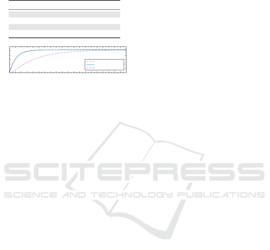
Table 2: Thermophysical properties of the freezer enclo-
sure.
Value Unit
Thermal conductivity, k 0.01 W/(mK)
Heat transfer coefficient, h 8 W/(m
2
K)
Specific heat capacity, c
p
650 J/(kgK)
Density, ρ 186 kg/m
3
Time [h]
0 10 20 30 40 50 60 70 80 90 100 110 120 130 140 150 160 170 180 190 200
Temperature [°C]
-80
-60
-40
-20
0
20
40
Manufacturer pull-up curve
Simulation, no load
Simulation, with load
Figure 4: Pull-up system response comparison.
3.2 Freezer Model Validation
In order to validate our model, we compared a simu-
lation of the freezer response without any load nor
contributions from the refrigeration system with the
freezer pull-up curve from the manufacturer. The sy-
stem response simulation in Figure 4 is shown in a
solid blue line against the manufacturer data, plotted
as a dashed red line. There is a very good match be-
tween the manufacturer data and simulation results,
which means that the model is sufficiently accurate
for our purposes. The figure shows that the time con-
stant of the system is approximately 70 hours with an
empty freezer. Our results are also in the same order
of magnitude, but comparatively higher than those in
refrigerators for residential applications, where a time
constant of approximately 20-30 hours is found (Ver-
zijlbergh and Lukszo, 2013). Figure 4 also compares
the pull-up system response under no-load conditions
(solid blue line) against the fully-loaded freezer with
blood samples described in the previous subsection
(purple dash-dotted line). It can be seen from the fi-
gure that the time constant of the system increases al-
most threefold, going from 70 hours in the no-load
case to 200 hours in the fully-loaded case, which is as
expected.
We also simulated the performance of the free-
zer under no-load conditions and compared it against
the electricity consumption given by the manufactu-
rer. Simulation results under no-load conditions show
that the daily electricity consumption of the freezer is
12.4 kWh/day. This represents a 7% error difference,
but is nevertheless a good, if conservative, approxi-
mation of the freezer’s cooling capacity that will take
into account future degradation of the freezer’s me-
chanical refrigeration system that comes with normal
use.
4 RESULTS
This section presents the simulation results for the
BAU scenario, plus the energy amount, energy cost,
and peak reduction optimizations. Due to the heuris-
tic nature of the GA, a number of local minima were
found in successive runs, and the best results are re-
ported graphically in Figs. 5-8, and are summarized
and compared against each other in Table 3.
4.1 BAU Scenario
Simulation results for the BAU scenario are shown
in Figure 5, which contains three subplots. The top-
most subplot (a) shows freezer contents (blue solid
line) and indoor temperatures (red solid line) with re-
spect to time. The middle subplot (b) shows whether
the mechanical refrigeration system is switched on at
every time step. Finally, the bottom subplot (c) shows
the electrical power consumption with respect to time
in a scenario with local PV generation, with positive
values denoting consumption and negative values de-
noting generation.
Results show that local PV generation by itself has
a beneficial effect on cost and energy reduction. Ho-
wever, it is possible to see from Figure 5(c) and Table
3 that an uncontrolled PV production has an adverse
effect in the system, in the form of a 5% increase in
the peak load from 132 to 139 kW.
4.2 Optimization Results
Optimization results are shown in Figure 6, Figure 7
and Figure 8 for the energy, cost, peak power mini-
mization objectives, respectively. The subplots and
legends for all optimization results are analogous to
those of Figure 5. In subplot (a), Ti
blood
denotes the
temperature of the blood samples of cluster i of inde-
pendently controllable freezers. The DR scheduling
process took approximately one and a half hours to
converge for each run in the MATLAB/Simulink si-
mulation environment.
The energy minimization objective is apparent in
Figure 6(b), since net energy exchanges with the elec-
tricity grid during times of solar energy production
are kept as close to zero as possible. The ability to
reduce the cooling load without infringing upon the
thermal safety boundaries is due to the freezers’ ther-
mal mass; i.e., the summation of the heat capacities
of the different freezer enclosure elements and their
contents: term (mc
p
)
x
in (1). Because of this need to
keep grid imports and exports to a minimum, the PV
utilization rate goes down to 77% with respect to the
uncontrolled BAU scenario with PV. Energy and cost
Demand Response of Medical Freezers in a Business Park Microgrid
125

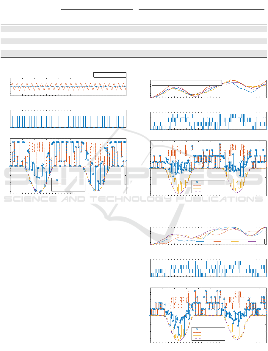
Table 3: Optimization results vs BAU scenario.
Energy [kWh] [AC] [%]
Scenario Imports Exports
Total
exchange
Social
cost
Cost
savings
Energy
savings
Peak
reduction
PV
utilization
BAU, no PV 3369.3 0 3369.3 92.89 — — — 0
BAU + PV, no DR 2235.1 793.2 3028.3 59.15 36 10 -5 100
Energy optimization 1482.1 35.1 1517.2 40.11 57 55 0 77
Cost optimization 1423.8 280.6 1704.4 36.92 60 49 0 88
Peak load optimization 2158.7 138.5 2297.2 58.37 37 32 25 50
0 5 10 15 20 25 30 35 40 45
Temperature [°C]
-85
-80
-75
(a) Temperatures
T
blood
T
in, air
0 5 10 15 20 25 30 35 40 45
β
0
1
(b) Mechanical heating/cooling switch
Time [h]
0 5 10 15 20 25 30 35 40 45
Power [W]
× 10
5
-1.5
-1
-0.5
0
0.5
1
1.5
(c) Electrical Power Consumption and Generation
Net power
Consumption
Local generation
Max. available DG-RES
Figure 5: Results for the BAU scenario + DG-RES, no DR.
savings are 55% and 57% respectively; however, this
optimization objective does not have any noticeable
effect on peak reduction.
From Table 3, although net energy consumption
is higher in the cost optimization scenario, cost per-
formance slightly improves, signifying a reduction of
60% with respect to the BAU scenario. Results in
Figure 7(c) show that consumption concentrates not
only on the times where the electricity prices are low,
but also where PV production is highest. As can be
seen in Table 3, the PV utilization rate is 12% less
than in the BAU case with uncontrolled PV genera-
tion and no DR.
The peak power minimization objective does pre-
cisely what it is supposed to do, keeping at most three
freezer clusters on at the same time or having all four
clusters on at times where PV is being produced to
keep peak power as low as possible. This scenario had
the lowest energy and cost savings performance of
the three optimization objectives studied in this work.
However, the results obtained for the peak minimiza-
0 5 10 15 20 25 30 35 40 45
Temperature [°C]
-80
-75
-70
(a) Temperatures
T1
blood
T2
blood
T3
blood
T4
blood
0 5 10 15 20 25 30 35 40 45
β
0
1
2
3
4
(b) Mechanical heating/cooling switch
Time [h]
0 5 10 15 20 25 30 35 40 45
Power [W]
× 10
5
-1.5
-1
-0.5
0
0.5
1
1.5
(c) Electrical Power Consumption and Generation
Net power
Consumption
Local generation
Max. available DG-RES
Figure 6: Results for energy minimization.
0 5 10 15 20 25 30 35 40 45
Temperature [°C]
-80
-75
-70
(a) Temperatures
T1
blood
T2
blood
T3
blood
T4
blood
0 5 10 15 20 25 30 35 40 45
β
0
1
2
3
4
(b) Mechanical heating/cooling switch
Time [h]
0 5 10 15 20 25 30 35 40 45
Power [W]
× 10
5
-1.5
-1
-0.5
0
0.5
1
1.5
(c) Electrical Power Consumption and Generation
Net power
Consumption
Local generation
Max. available DG-RES
Figure 7: Results for cost minimization.
SMARTGREENS 2018 - 7th International Conference on Smart Cities and Green ICT Systems
126

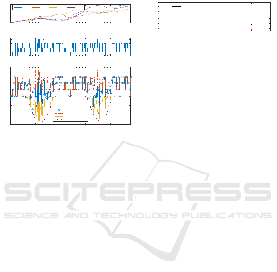
0 5 10 15 20 25 30 35 40 45
Temperature [°C]
-80
-75
-70
(a) Temperatures
T1
blood
T2
blood
T3
blood
T4
blood
0 5 10 15 20 25 30 35 40 45
β
0
1
2
3
4
(b) Mechanical heating/cooling switch
Time [h]
0 5 10 15 20 25 30 35 40 45
Power [W]
× 10
5
-1.5
-1
-0.5
0
0.5
1
1.5
(c) Electrical Power Consumption and Generation
Net power
Consumption
Local generation
Max. available DG-RES
Figure 8: Results for peak minimization.
tion objective still outperform those for the BAU with
uncontrolled PV scenario, with the added benefit of
reducing net peak power by 25%: a benefit that is ex-
tended not only for the microgrid consumers’ capacity
connection fees but also to the network operator, as
network reinforcements due to increased loads can be
delayed (although in this case study it is not a critical
problem).
Figure 9 shows the distribution of fitness function
values from all the successive simulation runs for each
optimization variant. They are expressed as the diffe-
rence with respect to the results from the BAU scena-
rio. Mean values for the simulation successions per-
formed for this work were (46 ± 8)% for the energy-,
(56 ± 2)% for the cost minimization, and (21 ± 6)%
for the peak reduction variants.
5 DISCUSSION
The results presented in the previous section show
the potential of implementing both price-responsive
(cost minimization) and direct control (peak load mi-
nimization) DR programs to harness flexibility from
C&I customers’ thermostatic loads. The benefits of
harnessing this flexibility are clear and attractive, in
terms of reductions in the amount and overall cost of
electricity demand for the end-users connected to the
microgrid. In the case of peak load reduction, pos-
sible deferrals in network reinforcement investments
and/or lower connection costs are also present. This
assertion holds for comparisons against both the BAU
scenario with no DG-RES and the BAU scenario with
Energy optimization Cost optimization Peak reduction
Difference vs. BAU [%]
10
20
30
40
50
60
Figure 9: Distribution of fitness function values for each
optimization variant.
DG-RES but no demand response. The benefits of
combining DR with customer thermostatic loads and
local DG-RES available in the microgrid is especially
evident when comparing results in terms of peak load
mitigation with respect to the BAU scenario with un-
controlled PV.
To put things in a realistic perspective, it is im-
portant to mention that the 55% energy savings in the
freezers’ operation translates overall to 19% energy
savings in the total electricity consumption of the me-
dical research facility. This number could be increa-
sed if, apart from the freezers, we could harness flex-
ibility from other thermostatic loads such as heating
and air conditioning systems in the rest of the medi-
cal research facility.
However, while achieving these targets, the ther-
mal inertia of the freezers is depleted at the end of the
48-hour window, since the freezer temperatures are
all at or near the temperature upper bounds of -70
◦
C
(see Figures 6(a) and 7(a)). This means that some re-
covery time is required immediately after the 48-hour
window where DR was implemented, during which
the freezers can recharge their thermal buffers (i.e.,
cool down to -80
◦
C). In order to overcome this limi-
tation, we will add end-of-horizon temperature targets
in the problem formulation in future versions of this
work to limit the state of charge of the thermal buffers.
Another limitation of our model is that the gre-
ater energy efficiency and lower demand/generation
peaks in the C&I microgrid —while being in the in-
terest of the microgrid as a whole— come at a loss
for the local PV producer. This is because PV uti-
lization rates become lower in the energy- and peak
load minimization objectives due to PV curtailment.
Since the two aforementioned optimization objectives
do not take price into account, a way to increase PV
utilization in these scenarios would be to add utiliza-
tion constraints linked to the target payback time or
return on investment for the PV producer. Similarly,
in order to decrease peak load, we could include peak
capacity tariffs in the objective function for the energy
and cost minimization variants.
We decided to study a 48-hour window to observe
the long-term temperature dynamics of the medical
freezers, given the high time constant of the system.
Additionally, we tested the robustness of our DR fra-
Demand Response of Medical Freezers in a Business Park Microgrid
127

mework with this expanded time window, since the
optimization problem increases in complexity given
the doubled number of design variables with respect
to observing a 24-hour window.
However, in practice it makes more sense to cre-
ate schedules on a day-ahead basis because electricity
prices would be known to the aggregator 24-hours in
advance and the performance of PV production fo-
recasting models improves the closer they are used
to the period of interest. More local DG-RES can
be installed in the business park if additional hea-
ting/cooling systems in the buildings located there can
be harnessed in the same way we have presented in
this paper without changing the network infrastruc-
ture. Scaling up or down our thermodynamic models
and DR framework —depending on the size of the
window, the time granularity, and the number of con-
trollable devices— should therefore present no signi-
ficant challenges when performing simulations.
Additional work is needed in order to surmount
some of the assumptions made when computing the
optimal schedules, especially with regards to dealing
with errors in the PV forecasting data. Further steps
are required in order to move out of the simulation
environment and into the practical implementation of
the proposed DR framework in the actual customer
site, especially considering that the current conver-
gence time is quite long. Optimizing the GA imple-
mentation in MATLAB in future versions of our work
will be essential to maintain the computation time be-
low the 24-hour window in which the DR scheduling
has to be made, especially when more sources of flex-
ibility are harnessed from the microgrid customers.
Because of the non-linear, combinatorial nature of the
optimization problems that make up our DR frame-
work, the heuristic methods used to solve them re-
quire multiple successive simulation runs from which
the best local optima can be selected. That is, de-
pending on the number of flexible sources/consumers
in the microgrid, it would be necessary to curtail the
computation time so as not to take longer than the
available scheduling window, at the expense of fin-
ding a better solution (see Figure 9).
6 CONCLUSIONS
This work modeled and optimized the thermodyna-
mic behavior of medical freezers in a research facility
in order to quantify their potential for DR programs.
In summary, the results presented show that flexibility
can be harnessed from the thermal mass of the free-
zers’ enclosure and contents, resulting in significant
benefits in terms of cost and energy efficiency for the
end-user. Although uncontrolled DG-RES is already
a significant benefit in terms of energy efficiency and
cost with respect to the BAU scenario, adding DR has
the following benefits: 1) reduces the coincidence of
the loads, 2) improves cost and energy performance
for the consumer; and 3) mitigates increased peak
loads due to uncontrolled in-feed of DG-RES at the
point of common coupling between the local business
park microgrid and the regional distribution grid.
Future work will extend the scope of our proposed
DR framework to the rest of the business park where
the medical freezing warehouse is located, in order
to combine the flexibility of the freezers in the medi-
cal research facility with other sources of flexibility
available: other buildings and their heating/cooling
systems, thermal buffers, and eventually electric vehi-
cles.
ACKNOWLEDGMENTS
Rosa Morales Gonz
´
alez would like to thank Julian
Croker for providing information on the case study,
and Cees Jan Dronkers for his constructive insight on
the interpretation of results.
REFERENCES
Alizadeh, M. I., Parsa Moghaddam, M., Amjady, N., Siano,
P., and Sheikh-El-Eslami, M. K. (2016). Flexibility
in future power systems with high renewable penetra-
tion: A review.
Ashok, S. and Banerjee, R. (2000). Load-management
applications for the industrial sector. Appl. Energy,
66(2):105–111.
ASM Aerospace Specification Metals Inc. AISI Type 304
Stainless Steel.
Centraal Bureau voor de Statistiek (2017a). Energiever-
bruik; opbouw, bedrijfstak.
Centraal Bureau voor de Statistiek (2017b). Monitor top-
sectoren 2017.
Compendium voor de Leefomgeving (2017). Bruto toege-
voegde waarde en werkgelegenheid, 1995-2016.
D’hulst, R., Labeeuw, W., Beusen, B., Claessens, S., De-
coninck, G., and Vanthournout, K. (2015). Demand
response flexibility and flexibility potential of residen-
tial smart appliances: Experiences from large pilot test
in Belgium. Appl. Energy, 155:79–90.
Eftekhar, J. G. (1989). Some Thermophysical Properties of
Blood Components and Coolants for D5U. Technical
report, University of Texas San Antonio, San Antonio.
European Environment Agency (2017). Final energy con-
sumption by sector and fuel.
Finn, P. and Fitzpatrick, C. (2014). Demand side manage-
ment of industrial electricity consumption: Promoting
SMARTGREENS 2018 - 7th International Conference on Smart Cities and Green ICT Systems
128

the use of renewable energy through real-time pricing.
Appl. Energy, 113:11–21.
Gela
ˇ
zanskas, L. and Gamage, K. A. A. (2016). Distributed
Energy Storage Using Residential Hot Water Heaters.
Energies, 9(3):127.
Gr
¨
unewald, P. and Torriti, J. (2013). Demand response from
the non-domestic sector: Early UK experiences and
future opportunities. Energy Policy, 61:423–429.
He, X., Keyaerts, N., Azevedo, I., Meeus, L., Hancher,
L., and Glachant, J.-M. (2013). How to engage con-
sumers in demand response: A contract perspective.
Util. Policy, 27:108–122.
Hewicker, C., Hogan, M., and Mogren, A. (2012). Po-
wer Perspectives 2030: On the road to a decarbonised
power sector. Technical report, Roadmap 2050, Den
Haag.
Huber, M., Dimkova, D., and Hamacher, T. (2014). Integra-
tion of wind and solar power in Europe: Assessment
of flexibility requirements. Energy, 69:236–246.
Hurtado, L., Mocanu, E., Nguyen, P., and Kling, W. (2015).
Comfort-constrained demand flexibility management
for building aggregations using a decentralized appro-
ach. In SmartGreens 2015 - 4th Int. Conf. Smart Cities
Green ICT Syst., pages 157–166, Lisbon.
Hurtado, L. A., Mocanu, E., Nguyen, P. H., Gibescu, M.,
and Kamphuis, I. G. (2017). Enabling cooperative be-
havior for building demand response based on exten-
ded joint action learning. IEEE Trans. Ind. Informa-
tics, PP(99):1.
Kalsi, K., Chassin, F., and Chassin, D. (2011). Aggregated
modeling of thermostatic loads in demand response:
A systems and control perspective. In Decis. Cont-
rol Eur. Control Conf. (CDC-ECC), 2011 50th IEEE
Conf., pages 15–20, Orlando. IEEE.
Klaassen, E., Frunt, J., and Slootweg, J. (2014). Method for
Evaluating Smart Grid Concepts and Pilots. In IEEE
Young Res. Symp. 2014 (YRS 2014), pages 1–6, Ghent.
EESA.
Labeeuw, W., Stragier, J., and Deconinck, G. (2015). Po-
tential of Active Demand Reduction With Residential
Wet Appliances: A Case Study for Belgium. IEEE
Trans. Smart Grid, 6(1):315–323.
Lampropoulos, I., Kling, W. L., Ribeiro, P. F., and van den
Berg, J. (2013). History of demand side management
and classification of demand response control sche-
mes. 2013 IEEE Power Energy Soc. Gen. Meet., pages
1–5.
Liu, W., Wu, Q., Wen, F., and Ostergaard, J. (2014). Day-
Ahead Congestion Management in Distribution Sys-
tems Through Household Demand Response and Dis-
tribution Congestion Prices. Smart Grid, IEEE Trans.,
5(6):2739–2747.
Ma, K., Hu, G., and Spanos, C. J. (2015). A Coope-
rative Demand Response Scheme Using Punishment
Mechanism and Application to Industrial Refrige-
rated Warehouses. IEEE Trans. Ind. Informatics,
11(6):1520–1531.
Maharashtra State Blood Transfusion Council (2014). Pre-
servation and Storage of Blood.
Matthews, B. and Craig, I. (2013). Demand side mana-
gement of a run-of-mine ore milling circuit. Control
Eng. Pract., 21(6):759–768.
MatWeb (2017). Unifrax Excelfrax 200 VIP Vacuum Insu-
lation Panel.
Mitra, S., Sun, L., and Grossmann, I. E. (2013). Opti-
mal scheduling of industrial combined heat and power
plants under time-sensitive electricity prices. Energy,
54:194–211.
Morales Gonz
´
alez, R., Shariat Torbaghan, S., Gibescu, M.,
and Cobben, S. (2016). Harnessing the Flexibility of
Thermostatic Loads in Microgrids with Solar Power
Generation. Energies, 9(7):547.
Samad, T. and Kiliccote, S. (2012). Smart grid technolo-
gies and applications for the industrial sector. Comput.
Chem. Eng., 47:76–84.
Ton, D. and Smith, M. (2012). The U.S. Department of
Energy’s Microgrid Initiative. Electr. J., 25(8):84–94.
Verzijlbergh, R. and Lukszo, Z. (2013). Conceptual model
of a cold storage warehouse with PV generation in a
smart grid setting. In 2013 10th IEEE Int. Conf. Net-
working, Sens. Control. ICNSC 2013, pages 889–894,
Evry. IEEE.
Wessling, F. and Blackshear, P. (1973). The Thermal Pro-
perties of Human Blood During the Freezing Process.
Heat Transf., 95(2):246–249.
Wilson, M. B., Luck, R., and Mago, P. J. (2015). A
First-Order Study of Reduced Energy Consumption
via Increased Thermal Capacitance with Thermal
Storage Management in a Micro-Building. Energies,
8:12266–12282.
Yin, R., Kara, E. C., Li, Y., DeForest, N., Wang, K., Yong,
T., and Stadler, M. (2016). Quantifying flexibility of
commercial and residential loads for demand response
using setpoint changes. Appl. Energy, 177:149–164.
Yoon, J. H., Baldick, R., and Novoselac, A. (2014). Dy-
namic Demand Response Controller Based on Real-
Time Retail Price for Residential Buildings. IEEE
Trans. Smart Grid, 5(1):121–129.
Zaparoli, E. L. and de Lemos, M. (1996). Simulation of
Transient Response of Domestic Refrigeration Sys-
tems. In Int. Refrig. Air Cond. Conf., pages 495–500,
West Lafayette. Purdue University.
Zavala, V. M. (2013). Real-time optimization strategies for
building systems. Ind. Eng. Chem. Res., 52(9):3137–
3150.
Demand Response of Medical Freezers in a Business Park Microgrid
129