Automatic Fault Detection using Cause and Effect Rules for In-vehicle

Networks

Alexander Kordes, Sebastian Wurm, Hawzhin Hozhabrpour and Roland Wism

uller

Operating Systems & Distributed Systems, University of Siegen, H

olderlinstraße 3, Siegen, NRW, Germany

Keywords:

Cause and Effect Rules, Machine Learning, In-vehicle Sensor Network, Fault Detection.

Abstract:

In-vehicle networks (IVNs) connect Electronic Control Units (ECUs) for automotive applications. Most of

the communication on the IVNs directly affect the comfort or even the safety of the driver. Therefore, it is

necessary to monitor these systems in order to ﬁnd the cause and effect of a fault. Current developments

use plausibility checks in automotive ECUs to enhance safety and security. Within the LEICAR project in

cooperation with INVERS GmbH we focus on all sensors signals recorded directly from CAN bus IVNs for

this positional paper. Even without the knowledge of the sensors semantics it is possible to extract cause and

effect rules for all recorded sensor signal relationships of the vehicle, map them in a graph and extract certain

situations. The proposed solution detects direct and slowly evolving changes even if they propagate across

several involved sensor values. For the automatic fault containment we extract features from the cause and

effect rules to train a machine learning model in order to make predictions on new data. Besides that it is

possible to implement optimized error checking procedures for the involved ECUs.

1 INTRODUCTION

Robust fault detection is a stringent requirement for

the evaluation of safety-critical applications on in-

vehicle networks (IVNs). Unfortunately, the search

space in recorded IVN sensor data increases with the

number of sensors mounted to the vehicle. In terms

of autonomous driving the number of involved sen-

sors and actuators increases with every new vehicle

model. Sensors and actuators are connected to elec-

tronic control units (ECUs) which transmit the sensor

data over the internal network. Therefore, the auto-

motive engineers of vehicle manufacturers spend a lot

of time with manual fault detection for vehicle proto-

types, if the faults are not detected by the on-board

diagnostics (OBD), which only performs plausibility

checks on the sensor data. However, faults effecting

the causal relationship between the sensor signals in

the IVN, which are not detected by the OBD, may oc-

cur during the machine life of a vehicle. These faults

can propagate through the IVN and need knowledge

about the whole system, to ﬁnd the cause of them. It

should be mentioned that the detection of faults, that

occur but just affect the system slowly over a long

period of time, like mechanical wear, is very time-

consuming for vehicle repair shops.

This is why we focus in this paper on a method

for automatic situation detection, in order to reduce

the search space for the automotive engineers. It is a

part of the LEICAR project

. The method presented

in this paper is adapted from (Hira and Deshpande,

2016) and adjusted by us in order to manage IVN

sensor data instead of socio-economic indicators, like

in the original method. We calculate causal relation-

ships between sensors, to obtain features for an au-

tomatic fault detection with machine learning algo-

rithms. This is veriﬁed with simulation and real IVN

data in which we ﬁrst detect situations and later per-

form automatic fault detection. In the future it could

be possible to integrate better fault detection mech-

anisms in the vehicle using the outcome of the pro-

posed method.

This conceptional paper is organized as follows:

We describe the relevant parts of the method of mod-

eling cause and effect rules for socio-economic indi-

cators in Section 2. In Section 3, we state the prob-

lems consisting of applying cause and effect rules to

IVN sensor data and extending the rules for automatic

fault containment. The related work is shown in Sec-

tion 4. In Section 5, we present the proposed method

based on the creation of extended cause and effect

Partially funded by German Federal Ministry of Edu-

cation and Research (BMBF).

Kordes, A., Wurm, S., Hozhabrpour, H. and Wismüller, R.

Automatic Fault Detection using Cause and Effect Rules for In-vehicle Networks.

DOI: 10.5220/0006792605370544

In Proceedings of the 4th International Conference on Vehicle Technology and Intelligent Transport Systems (VEHITS 2018), pages 537-544

ISBN: 978-989-758-293-6

537

rules and their visualization. We also discuss de-

tectable faults and the limits of the proposed method.

The effectiveness of the method is reviewed in Sec-

tion 6 using simulated and real data of a vehicles brak-

ing situations. We conclude this paper in Section 7.

2 EXTRACTION OF CAUSE AND

EFFECT RULES

For a better understanding, we will brieﬂy discuss the

most important aspects of the calculation of binary

cause and effect rules described in (Hira and Desh-

pande, 2016). The approach is used to model the de-

picted relationships in Figure 1 between various stock

market prices. The arrows in Figure 1 indicate a re-

lationship in the sense of a cause and effect rule be-

tween the two time series P

and P

. The arrow points

from the cause to the effect and if the cause occurs,

the effect takes place after a time lag ` > 0. The time

series of the stock market prices in (Hira and Desh-

pande, 2016) have one sample per year.

CyclicTransitive

Binary

Many to one

Figure 1: Causal relationships.

For the extraction of cause and effect relationships

it is necessary to calculate the rate of change (ROC)

per time series ﬁrst. The ROC is an extension of

the momentum, which is a simple technical analysis

where indicators show the difference between, e.g.,

today’s closing price and the close n days before. The

ROC is expressed as a ratio between a change in one

time series relative to a corresponding change in an-

other. Graphically, the ROC is represented by the

slope of a line.

To identify relationships between two time series

and P

, ﬁrst the ROC γ

i,k

of every time series P

the k − th year is calculated. δ deﬁnes the minimum

ROC used to consider a signiﬁcant change. In (1)

each time series value is categorized as a positive

ROC (U), a negative ROC (D) or no ROC (Q). The

type of change R

i,k

is deﬁned as follows:

i,k











U if γ

i,k

≥ δ

D if γ

i,k

≤ −δ

Q if −δ ≤ γ

i,k

≤ δ

(1)

The result from equation (1) is used to calculate the

strongest relationship between two time series with

a time lag `. The direct relationship D

i, j,k,`

between

two time series P

and P

, regarding to a time lag `, is

calculated according to:

i, j,k,`











1 if(R

i,k

= U ∧ R

j,k+`

= U)∨

i,k

= D ∧ R

j,k+`

= D)

0 otherwise

(2)

In case of the direct relationship, if the rate of change

of P

matches with the rate of change of P

after a time

period `, the support count of the direct relationship is

deﬁned as:

,`) =

n−`

∑

k=1

i, j,k,`

(3)

The support percent of the direct relationship between

and P

is deﬁned as:

,`) =

,`)

n − `

(4)

Thus, the temporal direct relationship between two

time series P

and P

for a time lag ` is deﬁned in (5),

with α

deﬁned as the threshold for all causal rela-

tionships.

−→ P

if α

≥ α

(5)

The inverse relationship I is deﬁned as:

i, j,k,`











1 if(R

i,k

= U ∧ R

j,k+`

= D)∨

i,k

= D ∧ R

j,k+`

= U)

0 otherwise

(6)

The support count S

is deﬁned as:

,`) =

n−`

∑

k=1

i, j,k,`

(7)

Thus, the support percent of indirect relationship α

is deﬁned as:

,`) =

,`)

n − `

(8)

The strength of the relationship Θ

is deﬁned as:

) = α · log(n), where

α = α

,`) or α

,`)

(9)

The count of the number of pairs when no rate

of change in P

is associated with positive or neg-

ative rate of change in P

after a time period `

is called neutral-change C

,`). The count

for the inverse relationship is called change-neutral

,`) and the count for a neutral ROC is called

neutral C

,`). The deﬁnitions should be taken

from (Hira and Deshpande, 2016).

With the calculated relationships, the temporal

odds ratio TOR is deﬁned. The direct odds ratio OR

VEHITS 2018 - 4th International Conference on Vehicle Technology and Intelligent Transport Systems

538

and the temporal indirect odds ratio OR

between two

time series P

and P

for a time lag ` are deﬁned as:

,`) =

,`) ·C

,`)

,`) ·C

,`)

(10)

,`) =

,`)

,`) ·C

,`)

(11)

If the result of a neutral relationship C

,`),

,`) or C

,`) between two time series

and P

is zero, it is considered as one to avoid an

inﬁnite temporal odds ratio TOR.

According to (Hira and Deshpande, 2016) a bi-

nary rule set (BRS) exists between P

and P

if there

is a temporal association rule P

−→ P

and OR

≥ β

or OR

≥ β, where β is the threshold for the tempo-

ral odds ratio TOR. The BRS is deﬁned as a tupel

BRShP

,y,`, α,T ORi, with the names of the time

series P

and P

, the trend y, direct D or inverse I, the

time lag `, the support percent of the relationship α

and the temporal odds ratio TOR.

The rules not explained here, are described in the

article (Hira and Deshpande, 2016) in more detail.

3 PROBLEM STATEMENT

Fault detection in IVNs sensor data currently does not

consider causal relationships to automatically ﬁnd de-

ﬁned situations of recorded vehicle data. A situation

recognition can reduce the search area if, for exam-

ple, an error occurs only in a certain driving situation,

such as a braking situation. The causal relationships

between sensor values can, on the one hand, indicate

errors in situations where they change or no longer ex-

ist, but on the other hand they can also be used to set

up dependency graphs between sensors. This makes

fault detection much easier for the expert.

In this positional paper we examine IVN sensor

data which are recorded on the CAN bus of a vehi-

cle or simulated for test purposes. A recording of a

trip is called a trace. We understand the individual

recorded sensors data as a single time series. The en-

tire recording is therefore taken as a set of time series

of the form T = {T

|i, j = 1,...,n}. When calcu-

lating causal rules, always two time series of set T , T

and T

are used for the method with T

6= T

During fault analysis in IVNs, currently there are

not enough causal rules to properly map the relation-

ships between all recorded sensor signals. The cause

and effect rules can be used to characterize various sit-

uations, to later identify them automatically in IVNs,

where faults have occurred. This limits the search

space for faults and can be used for visualization and

veriﬁcation using, e.g., a requirement speciﬁcation.

Extended cause and effect rules can also be used as a

feature for machine learning procedures in automatic

fault detection and fault prediction methods. In partic-

ular, changes that occur especially in the case of tem-

porally changing relationships between components

can be detected and predicted very effectively using

cause and effect relationships, as is the example of

mechanical wear in braking situation.

The recorded sensor signals from the IVN can ei-

ther be noisy and unmodiﬁed raw output from sensors

or pre-processed and fused signals. The IVNs sen-

sor signals could not have the same sampling rate and

therefore, cannot be compared directly at any time,

which is not the case in the example of stock mar-

ket prices (one sample per year). In order to calculate

cause and effect relationships from sensor signals, dif-

ferent pre-processing steps must be carried out ﬁrst,

to reduce noise and change their sampling rate to an

identical one by interpolation.

The next step is calculating the cause and effect

relationships for given situations. The strongest rela-

tionships between the sensors describe this particular

situation. To determine the correct mode of operation,

the rules have to be visualized and proven by expert

knowledge.

For the automatic detection of faults in certain sit-

uations, especially slightly changing relations over a

long period of time, the cause and effect rules have to

be extended in order to detect the situations of interest

and provide good features for training and subsequent

veriﬁcation of, e.g., a machine learning model.

4 RELATED WORK

Vehicles can be affected by a wide variety of faults.

In order to avoid personal injury it is of great inter-

est to detect critical faults as early as possible. How-

ever, according to (Rosich et al., 2012) simple plausi-

bility checks are carried out in many error diagnosis

systems, like the self-diagnostic and reporting system

(OBD) of a vehicle. These systems just check sen-

sor values against predeﬁned threshold values. There

are also improved methods of veriﬁcation like (Ko-

rte et al., 2012; Kordes et al., 2014; Deb et al., 2013).

Above all, not only individual sensors can be checked,

but also the entire sensor network of a machine can

be examined. However, in (Rosich et al., 2012) it is

pointed out that the complexity of methods should not

become so high that they are no longer practically ap-

plicable. Thus, it is necessary to use techniques to

model all causal relationships between all involved

time series and have exact knowledge of it, which re-

Automatic Fault Detection using Cause and Effect Rules for In-vehicle Networks

539

quires expert knowledge. In addition, this knowledge

must be used to create competing models, from which

the best is selected through system identiﬁcation.

To validate individual sensor values, the principal

component analysis is used by (Kerschen et al., 2005)

and artiﬁcial neural networks are used by (Xu et al.,

1999; Klimkowski, 2016). In the mentioned proce-

dures, only individual sensors are checked for fault-

lessness. This means that no relationships (causal-

ity) between the sensors are used to draw conclusions

about the entire system state or related sub-sections.

According to the current state of research, there

are several methods for including causality. The ap-

proach of (Tucker and Liu, 2004) describes how dy-

namic Bayesian networks, trained from existing sen-

sor data, are used to model the dependencies between

sensors as a dependency graph. This method is used

to visualize changes in the dependency structure and

thus identify faults. In the approach of (Alippi et al.,

2014) a dependency graph is created to ﬁnd relations

between sensors, based on the Granger causality con-

cept. The proposed statistical framework is then com-

bined with a hidden Markov model to ﬁnd and isolate

errors in the sensor network.

The proposed method of (Hira and Deshpande,

2016) for creating cause and effect rules is compared

to both, the Granger causality and the Bayesian net-

works. They conclude that their method is faster

and can determine not only binary but also transitive,

cyclic and many to one relations. Since we want to

model all possible causal relationships between sen-

sor signals, we will expand the described method and

apply it to IVNs.

5 PROPOSED SOLUTION

In this section we describe our analysis and imple-

mentation of an ofﬂine situation and fault detection

method for IVNs, based on the approach of (Hira and

Deshpande, 2016). It is extended by a pre-processing

step to handle IVN sensor signals and is corrected in

some places. In the current state of research, we only

use the calculation of the BRS

On the one hand, the calculation of cause and ef-

fect rules is used to create graphs with causal rela-

tionships of the sensors in various situations and on

the other hand, for the reduction of the search space

and further feature extraction for error detection. The

extracted features are used for training, test and val-

The future work consists among other things of mod-

eling all causal relationships presented in (Hira and Desh-

pande, 2016).

idation of a decision tree algorithm to automatically

detect faults.

In the following sections we describe the adjust-

ments to the original method of (Hira and Deshpande,

2016) and pre-processing steps for the use of IVN

sensor signals with it. Afterwards we describe our

method of situation learning in order to detect them

automatically in recorded traces. Finally, we discuss

certain fault detection methods for different faults.

5.1 Adjusting Cause and Effect Rules

for IVN Data

Generally, we follow the implementation of (Hira and

Deshpande, 2016). Instead of the ROC we use the

slope m

i,k

, to calculate the relationships between two

time series T

and T

. δ is redeﬁned to the minimum

slope to consider a signiﬁcant change and instead of

stings we use numerical values

to calculate the R

i,k

redeﬁned as:

i,k











1 if m

i,k

≥ δ

−1 if m

i,k

≤ −δ

0 if −δ ≤ m

i,k

≤ δ

(12)

Furthermore, the deﬁnition of the temporal inverse

odds ratio OR

deﬁned in 11 has been corrected by us,

using C

as a multiplier in the numerator, because the

odds ratio is the same calculation as the cross product

ratio deﬁned in (Mosteller, 1968). The new deﬁnition

of the temporal inverse odds ratio OR

is:

,`) =

,`) ·C

,`)

,`) ·C

,`)

(13)

Finally, we redeﬁned the BRS by deleting

the ROC and adding the mean of the slope µ

and the standard deviation of the slope σ to

BRShT

,y,`, α,T OR,µ, σi. These values are also

used as features for an automatic fault detection.

Further adjustments will be done in the future

work, if we add other causal relationship types to the

binary relationship, used in the proposed solution.

5.2 Pre-processing IVN Sensor Data

The starting point of our analysis is comparing the

features of time series from the stock market prices,

which are used as input for the cause and effect rule

modeling of (Hira and Deshpande, 2016) and time se-

ries from recorded test drives in IVNs in different sit-

uations like parking, braking, normal drive behavior

The use of numerical values is convenient for compu-

tation for large, multidimensional arrays.

VEHITS 2018 - 4th International Conference on Vehicle Technology and Intelligent Transport Systems

540

over short and longer time periods etc. The main dif-

ferences are: The time series of IVNs do not all have

the same sampling rate, they can have different reso-

lutions starting from one bit

up to several bytes, they

can have positive and negative values, they have a lot

more data points and they can be affected by noise.

Therefore, we implemented different pre-processing

steps.

First, we extract the sensor signals from the IVNs

recorded trace ﬁle as described in (Kordes et al.,

2018). The signals are re-sampled to construct new

data points within the range of the discrete set of

known data points of every sensor signal. To reduce

the noise of some signals, we use a low pass ﬁlter.

Figure 2 a) shows the original signal and b) shows

the smoothed signal

. After the pre-processing we

Time Time

Value

Figure 2: Low pass ﬁlter.

get a set of time series T = {T

,..., T

}. The pre-

processing has to be done just for IVN sensor data.

5.3 Situation Learning

A situation is described by the strongest relationships

between all involved sensor values during the period

of time, the situation occurs. In the current state of

research, we only use the BRSs as describing rela-

tionships. In case of IVN sensor data, we assume that

the pre-processing step has already been performed.

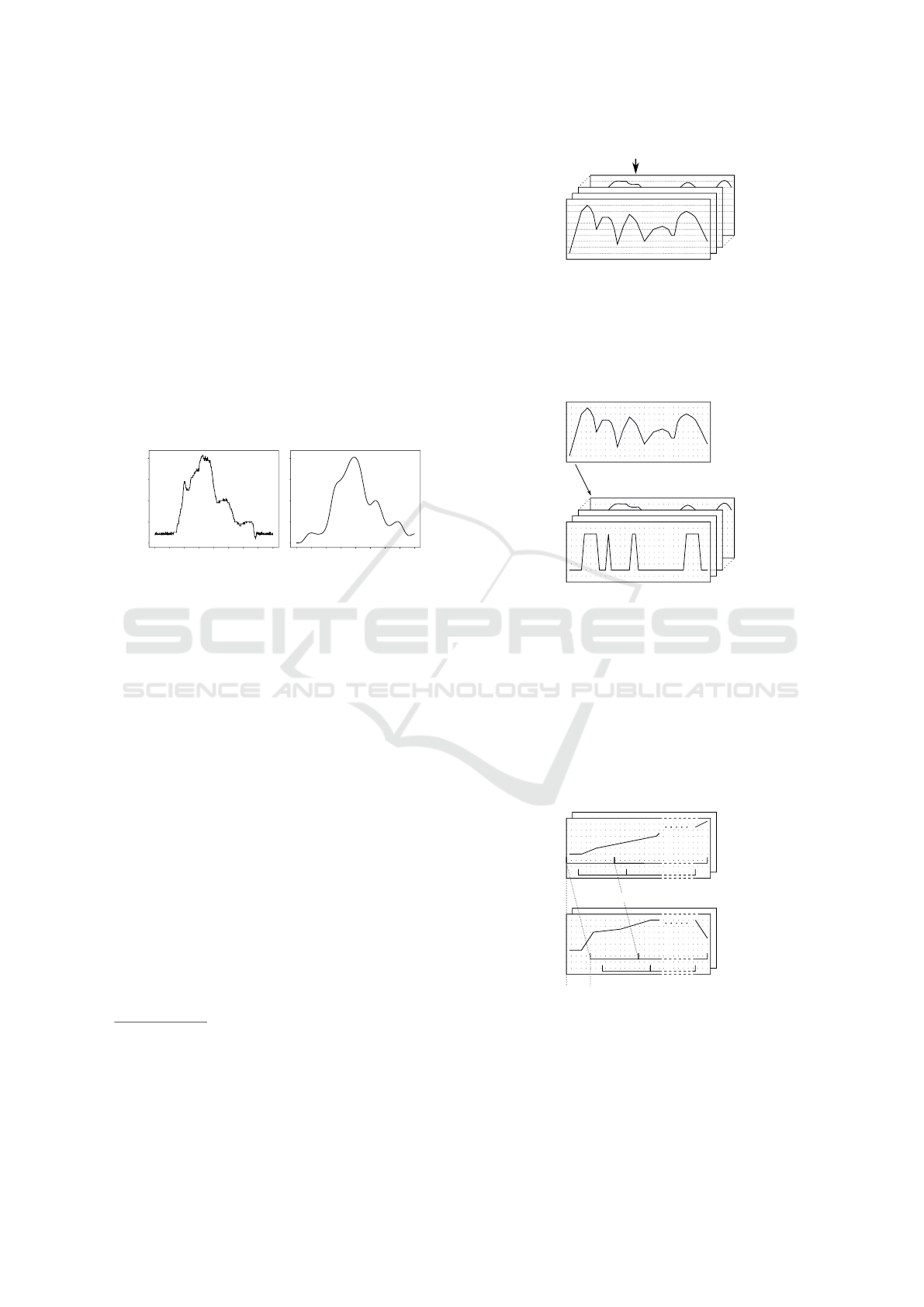
To automatically learn and detect certain situa-

tions, we follow the pipeline of situation learning

which is segmented in the four computing steps, time

series extraction, time lag calculation, BRS calcula-

tion and the optional step of graph visualization. In

the ﬁrst step of the pipeline, it is necessary to create a

simulation or record all involved sensors in a situation

of interest (or more than one) and extract the time se-

ries as set T = {T

,...T

}, as depicted in Figure 3.

After the extraction step, we compute causal rules

of all subsets of set T , with two differing elements

}, to determine the optimal time lag

` of the

Time series, which are only represented by binary val-

ues, have been ignored for simpliﬁcation in the proposed

method.

Noise detection is done manually.

To simplify matters, it is assumed that the requested sit-

uation corresponds to the total length of the recorded trace.

Time

Value

IVN or simulation

Figure 3: Time series extraction.

subsets. This second step of the pipeline is depicted

in Figure 4. We use a predeﬁned α

= −1 and β = −1

in order to ensure a BRS is calculated per compared

time series.

Time

Value

Time

Value

Compute BRS

Figure 4: Time lag calculation.

In the third step of the pipeline, we ﬁrst seg-

ment the time series T

into small sub windows of

equal length. The sub windows overlap each other

(sw

,..., sw

), like depicted in Figure 5. The time se-

ries T

is also segmented in sub windows starting with

an offset of time lag `, as calculated in the second step

of the pipeline. We now calculate the strongest BRS

with the longest sub sequence for all different sets of

and T

Time

Value

Time

Value

time lag ℓ

Compute BRS

Figure 5: BRS calculation.

Therefore, we ﬁrst compute a causal rule for

) and sw

). If k = 0 and we get a BRS

(α ≥ α

and T OR ≥ β), we increment k and go on

with the next sub window. Else if k > 0 and we get a

BRS for sw

) and sw

), we merge the actual sub

Automatic Fault Detection using Cause and Effect Rules for In-vehicle Networks

541

window sw

with the pre sub window sw

k−1

and cal-

culate a new BRS. We increment k and proceed with

the next sub window. The termination criteria for the

actual calculation are α < α

, T OR < β or the last sub

window of T

is reached. We get the strongest BRS

with the longest sub sequence for the sets T

and T

We perform this for all sets, until we have calculated

all BRSs

The fourth step of the pipeline is the optional vi-

sualization as a relationship graph. An example of a

relationship graph is depicted in Figure 6.

Figure 6: Example of relationship graph.

To detect the learned situation in a recorded driv-

ing behavior, we use the calculated causal relation-

ships with the deﬁned time lag ` and sub windows

like in step three of the pipeline of situation learning.

The difference is, that we compare each found BRS

with the BRSs of the learning phase. If it matches a

BRS of the learning phase, we try to ﬁnd the other

corresponding BRSs with the involved T

. If we get

the whole set of BRSs, we found the exact situation,

if it differs in small subset, this subset has to be re-

viewed for fault detection. Depending on the record-

ing, we start over with the next sub window, to ﬁnd

other situations of the same type.

The proposed solution is still work in progress.

In the current state of research we set values man-

ually, like the minimum slope δ, α

, β and the sub

window size used in the pipeline. The next step is to

improve the calculation steps of the pipeline, to make

the method more robust and more precise. Therefore

we can label the BRSs found within the positive situ-

ations recorded and use them as feature for a machine

learning algorithm (i.e., a support vector machine),

to identify the situations in new recordings, with no

knowledge about the content.

5.4 Fault Detection

The situation recognition is carried out as pre-

processing so that only the situations itself can be an-

The method will be adjusted in order to make it more

robust.

alyzed for the fault detection.

Faults that affect the causal relationships can be

detected by simply comparing the causal relationship

graphs of positive and negative cases. In the case a

BRS is missing between two time series, it can be

the case if an ECU goes into a fault state and trans-

mits only a ﬁxed value or a short circut has occurred.

The causal relationship graph can be used by automo-

tive engineers to identify all affected relationships and

sensors, if a fault propagates through the IVN.

To detect an error that manifests itself in a tem-

poral offset, like a mechanical wear, we can use the

aforementioned BRSs with the new values of the µ

and σ as features for a supervised machine learning

algorithm. Therefore it is necessary to record positive

and negative examples in order to train the algorithm

and ﬁnd faults or slightly differing values over time, in

new recordings. With predictive modeling, we could

predict in the future.

There are also algorithms that detect unusual be-

havior (Shirahama et al., 2016). The proposed method

could be used as a pre-processing step in order to re-

duce the search space for such algorithms in the future

work.

6 EXPERIMENTAL RESULTS

In Section 5, we present the proposed situation detec-

tion method based on the creation of adjusted cause

and effect rules and their visualization. We also dis-

cussed detectable faults and the current limits of the

proposed method. The effectiveness of the method is

reviewed in this section using simulated and real data

of a vehicles braking situations.

6.1 Simulated Braking Situations

To evaluate the proposed method, an idealized decel-

eration is simulated. The required formulas are taken

from (Mitschke and Wallentowitz, 2014). It consists

of three different time series: velocity v, deceleration

a and distance traveled s. The simulation can be ini-

tialized with the threshold time and the friction coefﬁ-

cient. The range for positive or negative samples can

be taken from Table 1 which is a collection from (Bur-

ckhardt, 1991; Gomeringer et al., 2014). The situa-

tion detection described in Section 5 is not used be-

cause the whole simulation models only the situation

to be detected.

In the ﬁrst step the algorithm for computing BRSs

is used to determine the relationships between the

three time series. The resulting graph is shown in Fig-

ure 7.

VEHITS 2018 - 4th International Conference on Vehicle Technology and Intelligent Transport Systems

542

Table 1: Parameter of braking situation.

[s] a

max

[m/s

]

case min max min max V

[m/s]

pos. 0.14 0.18 0.76g 0.8g 13.88

neg. 0.19 0.30 0.75g 0.66g 13.88

Figure 7: Relationship graph for simulated brake situation.

The BRS calculated between s and v is grayed out,

because the distance can not be the cause of the veloc-

ity, thus expert knowledge is used to identify and dis-

card it. If we generate a negative brake situation, the

BRS sets are the same as in the positive case. Thus

we take µ and σ into account to identify this.

In the experiment we generate 200 positive and

200 negative braking situations by randomly assign-

ing equally distributed values from Table 1. For each

braking situation the three time series are generated.

We cut all of them at the minimum threshold time

of 0.14s, because else it is possible to distinguish

between the positive and negative situations by just

counting the data points of the time series.

Then for each braking situation the BRSs men-

tioned above are computed and labeled. For each type

of BRS a feature matrix is compiled, consisting of the

µ and σ as input for a machine learning model. In this

example a decision tree algorithm is used. The results

are the same for all BSRs and are cross validated (3-

Folds). This is shown in Table 2.

Table 2: Metrics.

class precision recall f1-score support

neg 1.00 1.00 1.00 200

pos 1.00 1.00 1.00 200

avg/total 1.00 1.00 1.00 400

The results are questioned, because 100% accu-

racy is reached and could be the cause of overﬁtting.

But if one examines the decision tree, it has only a

height of one. This means only the feature µ is used

to make the split between the cases. If we compute a

probability density function (PDF) of µ in the positive

and negative situations, we can separate very clearly

between the situations, shown in Figure 8. Therefore,

we can validate the result of the decision tree.

We conclude, in the simulated situation we get

very good results. This has to be validated with real

IVN data.

Probability

µ(a)

pos neg

-55 -50 -45 -35

-30

-25-40

0.00

0.20

0.40

0.60

0.80

1.00

Figure 8: Probability density function of µ(a).

6.2 Real Braking Situations from IVN

Sensor Data

The next step we evaluate the situation detection with

real IVN data of a Ford Fiesta MK-II. We recorded

CAN bus data for a test drive which contains several

braking situations to automatically detect only the sit-

uations braking from 20km/h down to 15k m/h. In

the recorded trace there are only positive examples of

a brake without mechanical wear.

With expert knowledge we modeled a sub graph

of involved time series during a brake situation. It

contains the veriﬁed relationships of the deceleration

sensor a, the velocity v and the brake pedal position b:

BRS

b→a

, BRS

b→v

and BRS

a→v

. An unﬁltered excerpt

of the time series is shown in Figure 9.

Value

Time [ms]

438000 440000 442000 444000

-40

-20

20 -> 15 km/h

Figure 9: IVN brake situation (Ford Fiesta MK-II).

The pre-processing steps described in section 5

are applied on the time series to eliminate noise and

re-sample them and the optimal time lag is deter-

mined by the proposed method. Next we applied

the veriﬁed relationships to the method in order to

ﬁnd braking situations in a trace of several minutes.

Through empirical tests a sub window size of 500ms

equivalent to 50 data points and a overlap of 25 data

points is used. The α-value is set to 90%. The result

is shown in Figure 10, where the brake situations are

marked between dashed lines. The proposed method

found every brake situation in the trace

We also modeled good and bad brake examples

using the IVN sensor data, depicted in the left-hand

Is veriﬁed by manual situation detection.

Automatic Fault Detection using Cause and Effect Rules for In-vehicle Networks

543

Values normalized

Time[ms]

48000 52000 56000 60000

0.2

0.3

0.4

0.5

0.6

0.7

0.8

0.9

0.1

Figure 10: Found IVN brake situations.

side of Figure 11

and got the result the PDF of µ(v)

on the right-hand side of Figure 11. The decision tree

has, like in the simulation, a depth of one. So the

PDFs were examined and result that even in the real

IVN sensor data, there are features with optimal se-

lectivity, like the µ(v).

Velocity in km/h

Pos

Neg

Normalized time

0.5 0.6 0.7 0.8 0.9 1.0

Pos Neg

0.0

0.2

0.4

0.6

0.8

1.0

Probability

1.2

µ(v)

-5.5 -4.5 -3.5 -2.5

Figure 11: Modeled brake examples and resulting PDF.

7 CONCLUSIONS

The experimental results show that the adjusted

method of (Hira and Deshpande, 2016) performs very

well with a simulated situation and situations derived

from real traces of IVN sensor data, shown in Sec-

tion 6. It is able to learn deﬁned situations and ﬁnd

them in unknown time series.

The automatic fault detection, in the case of me-

chanical wear, is veriﬁed with a positive result in a

simulated situation as well as in real traces of IVN

sensor data. Therefore we used positive examples

from test rides and modeled negative examples.

According to the results, the method of modeling

causal relationships between time series can be ap-

plied to sensor signals of IVNs very well. It has to be

adjusted in the future work in order to make it more

robust and decrease the cost in means of computation

time, by applying new techniques like machine learn-

ing algorithms in intermediate steps of the method.

All previously manually deﬁned variables have to be

decided automatically.

Samples are divided into small sub windows in order to

get more training data.

REFERENCES

Alippi, C., Roveri, M., and Trov, F. (2014). Learning causal

dependencies to detect and diagnose faults in sensor

networks. In 2014 IEEE Symposium on Intelligent

Embedded Systems (IES), pages 34–41.

Burckhardt, M. (1991). Fahrwerkstechnik: Bremsdynamik

und Pkw-Bremsanlagen. Vogel-Verlag.

Deb, A. K., Kordes, A., and Vermeulen, H. G. H. (2013).

Flexray network runtime error detection and contain-

ment. US Patent 20140047282A1.

Gomeringer, R., Heinzler, M., Kilgus, R., Menges, V.,

aher, F., Oesterle, S., Scholer, C., Stephan, A., and

Wieneke, F. (2014). Tabellenbuch Metall. Europa-

Fachbuchreihe f

ur Metallberufe. Europa-Lehrmittel.

Hira, S. and Deshpande, P. S. (2016). Mining precise cause

and effect rules in large time series data of socio-

economic indicators. SpringerPlus, 5(1):1625.

Kerschen, G., Boe, P. D., Golinval, J.-C., and Worden, K.

(2005). Sensor validation using principal component

analysis. Smart Materials and Structures, 14(1):36.

Klimkowski, K. (2016). An artiﬁcial neural networks ap-

proach to stator current sensor faults detection for

dtc-svm structure. Power Electronics and Drives, 1

(36)(1).

Kordes, A., Hozhabrpour, H., Wism

uller, R., and Grze-

gorzek, M. (2018). Vehicle-independent interpretation

of sensor signals without a-priori knowledge of their

semantics. In press, VDE GMM-Fachtagung AmE Au-

tomotive meets Electronics, Dortmund, Germany.

Kordes, A., Vermeulen, B., Deb, A., and Wahl, M. (2014).

Startup error detection and containment to improve

the robustness of hybrid ﬂexray networks. In Proceed-

ings of the conference on Design, Automation & Test

in Europe, page 5. European Design and Automation

Association.

Korte, M., Holzmann, F., Kaiser, G., Scheuch, V., and Roth,

H. (2012). Design of a Robust Plausibility Check for

an Adaptive Vehicle Observer in an Electric Vehicle,

pages 109–119. Springer Berlin Heidelberg, Berlin,

Heidelberg.

Mitschke, M. and Wallentowitz, H. (2014). Dynamik der

Kraftfahrzeuge. Springer Vieweg.

Mosteller, F. (1968). Association and estimation in con-

tingency tables. Journal of the American Statistical

Association, 63(321):1–28.

Rosich, A., Frisk, E., Aslund, J., Sarrate, R., and Nejjari, F.

(2012). Fault diagnosis based on causal computations.

IEEE Transactions on Systems, Man, and Cybernetics

- Part A: Systems and Humans, 42(2):371–381.

Shirahama, K., K

oping, L., and Grzegorzek, M. (2016).

Codebook approach for sensor-based human activity

recognition. In Proceedings of the 2016 ACM Interna-

tional Joint Conference on Pervasive and Ubiquitous

Computing: Adjunct. ACM.

Tucker, A. and Liu, X. (2004). A bayesian network ap-

proach to explaining time series with changing struc-

ture. Intell. Data Anal., 8(5):469–480.

Xu, X., Hines, J. W., and Uhrig, R. E. (1999). Sensor vali-

dation and fault detection using neural networks.

VEHITS 2018 - 4th International Conference on Vehicle Technology and Intelligent Transport Systems

544