Optimized Feature Selection for Initial Launch in Dynamic Software

Product Lines

Ismayle de Sousa Santos

, Evilasio Costa Junior

1,∗

, Rossana Maria de Castro Andrade

1,†

Pedro de Alc

antara dos Santos Neto

2,‡

, Leonardo Sampaio Rocha

3,§

, Claudia Maria Lima Werner

4,¶

and Jerffeson Texeira de Souza

Department of Computer Science, Federal University of Cear

a, Fortaleza, Brazil

Department of Computer Science, Federal University of Piau

ı, Teresina, Brazil

Science and Tecnology Center, State University of Cear

a, Fortaleza, Brazil

Computer Systems Engineering Program, Federal University of Rio de Janeiro, Rio de Janeiro, Brazil

werner@cos.ufrj.br

Keywords:

Software Product Line, Dynamic Software Product Line, Graph, Multi-objective Optimization.

Abstract:

A Dynamic Software Product Line (DSPL) allows the generation of products that can adapt dynamically

according to changes in requirements or environment at runtime. This runtime adaptation is often made by the

activation and deactivation of features, introducing a cost (e.g., an overhead regarding resource consumption).

To reduce this cost, a solution is the partial product conﬁguration at the static binding time. Thus, in DSPLs,

one challenge is the feature selection to deﬁne which features should be bound permanently before the initial

launch and which features should be bound at runtime. In this paper, we address this challenge presenting a

graph model formulation to the feature selection problem for the initial launch in DSPLs that considers both

static and dynamic binding. This model allows the application of efﬁcient optimization algorithms to solve

the problem. We also present a proof of concept showing that the model can be used to generate optimized

solutions to the feature selection problem for initial launch in DSPLs.

1 INTRODUCTION

A Software Product Line (SPL) is a reuse-oriented

approach that aims the development of products by

reusing common artifacts (Eriksson and Hagglunds,

2003). Despite the beneﬁts of an SPL, it cannot

handle the dynamic variations (at runtime) in user

requirements and product environment (Hallsteinsen

et al., 2008). To address this gap, Dynamic Software

Product Lines (DSPLs) emerged as an extension of

the concept of conventional SPLs, enabling the gene-

ration of software variants at runtime (Bencomo et al.,

2012).

In order to support dynamic variability, a DSPL

has multiple and dynamic binding (Capilla et al.,

2014). The binding time is the time at which one

∗

PhD scholarship (MDCC/DC/UFC), sponsored by CAPES

†

Researcher scholarship - DT Level 2, sponsored by CNPq

‡

Researcher scholarship - DT Level 2, sponsored by CNPq

Researcher scholarship - PQ Level 2, sponsored by CNPq

Researcher scholarship - PQ Level 1, sponsored by CNPq

decides to include or exclude a feature from a pro-

duct (Chakravarthy et al., 2008). According to Ro-

senm

uller et al. (Rosenm

uller et al., 2011), the static

binding occurs when a feature is bound in a program

before load time (e.g., at compilation time), whereas

the dynamic binding occurs at load time or after loa-

ding a program. In traditional SPL engineering, featu-

res are bound only statically. Thus, once the product

is generated from the SPL, it cannot longer be chan-

ged at runtime (Hallsteinsen et al., 2008). DSPLs, ho-

wever, can combine static and dynamic binding and,

therefore, their features can be bound several times

and at different time periods (Capilla et al., 2014).

Thus, DSPLs can produce software capable of

adapting to user needs and evolving resource con-

straints (Hallsteinsen et al., 2008). It is worth no-

ting that the static binding provides ﬁne-grained cu-

stomization without any inﬂuence on the resource

consumption, but it can result in a functional over-

head when features included in the product are not

used (Rosenm

uller et al., 2009). Dynamic binding,

in turn, provides more adaptability by dynamically

de Sousa Santos, I., Costa Junior, E., Andrade, R., de Alcântara dos Santos Neto, P., Sampaio Rocha, L., Maria Lima Werner, C. and Texeira de Souza, J.

Optimized Feature Selection for Initial Launch in Dynamic Software Product Lines.

DOI: 10.5220/0006778001450156

In Proceedings of the 20th International Conference on Enterprise Information Systems (ICEIS 2018), pages 145-156

ISBN: 978-989-758-298-1

145

loading features when required, but usually, intro-

duces an overhead regarding resource consumption

and performance, and increases the execution time

(Rosenm

uller et al., 2011)(Rosenm

uller et al., 2009).

Therefore, one partial DSPL product conﬁguration,

binding some of the variation points at design time,

can be done before the initial launch for dealing with

the trade-off between the advantages and disadvanta-

ges of each binding time.

In this scenario, the product conﬁguration pro-

blem is how to decide which features should be bound

only statically, before initial launch, and which featu-

res should be bound dynamically.

In a small SPL, it is feasible to use exact techni-

ques to solve the product conﬁguration problem based

on feature attributes (Olaechea et al., 2014). These at-

tributes specify extra-functional information such as

speed or RAM required to support the feature (Be-

navides et al., 2010). Meanwhile, in a medium or

large SPL, this solution can take a prohibitive time.

Then, the use of Search Based Software Engineer-

ing (SBSE), which refers to the use of computatio-

nal search as a mean of optimizing software engineer-

ing problems (Harman et al., 2014), can be neces-

sary to obtain an optimum solution in an acceptable

time. In fact, we agree with Lopez-Herrejon et al.

(Lopez-Herrejon et al., 2015) that “the product con-

ﬁguration naturally lends itself to the application of

SBSE techniques because of the vast number of com-

binations that SPL requirements can typically have”.

After an analysis of the literature (see Section 6),

we observed that the existing approaches did not ad-

dress the feature selection problem in DSPLs, before

the initial launch. Addressing this gap, this paper pro-

poses a multi-objective approach based on a graph

model for the feature model rules veriﬁcation. We

decide to use a graph approach, because it can facili-

tate the representation and understanding of the fea-

ture model rules, besides allowing the use of different

optimization algorithms to solve the feature selection

problem. Moreover, this approach is easily imple-

mentable, once that graphs are well-known structu-

res. There is already some SBSE approaches that mo-

del the feature selection problem using graphs (Wang

and Peng, 2014), but they are focused in SPL.

The main contributions of this paper are as fol-

lows:

• we present a graph model created from the fea-

tures model considering both static and dynamic

binding times. Any optimization algorithm can

be used with the proposed model to solve the fe-

ature selection problem for the initial launch in

dynamic software product lines; and

• we introduce a multi-objective generic formula-

Figure 1: An example of SPL feature model.

tion for the feature selection problem in a DSPL;

and

• we present a proof of concept performed to as-

sess the feasibility of using our proposal to ge-

nerate optimum solutions to the feature selection

problem for initial launch in DSPLs;

2 FEATURE MODEL

Features are attributes of a system that directly affect

end-users (Kang et al., 1990). In a feature model, the

features are presented in a hierarchical way, and the

basic rules are: (i) the root feature is included in all

products; (ii) a child feature can only be included in

a product if its parent feature is included; and (iii) a

variation point is a point in the feature model where a

choice needs to be made. Figure 1 shows an example

of SPL feature model, where the features Illumination

and Doors are variation points.

Usually, a feature model allows the following re-

lationships among features (Benavides et al., 2010):

(i) Mandatory, a child feature has a mandatory re-

lationship with its parent when the child is ad-

ded in all products in which its parent feature

appears;

(ii) Optional, a child feature has an optional relati-

onship with its parent when the child can be op-

tionally added in all products in which its parent

feature appears;

(iii) Xor, a set of child features has a Xor-relationship

with its parent when only one child feature can

be selected when its parent feature appears; and

(iv) Or, a set of child features has an Or-relationship

with its parent when one or more of them can

be included in the products in which its parent

feature appears.

A feature model can also contain cross-tree con-

straints speciﬁed by require and exclude relationships

between features (Benavides et al., 2010). In an SPL,

if a feature A excludes a feature B, then both features

ICEIS 2018 - 20th International Conference on Enterprise Information Systems

146

cannot be included in the same product. If a feature

A requires a feature B, then there is a dependence re-

lationship where if feature A is included in a product,

then feature B is also included.

It is worth noting that in a DSPL, a variation point

can be bind at runtime by (de)activating the features.

In this scenario, if a feature A excludes a feature B,

then these features cannot be active in the product at

the same time. Also, if a feature A requires a feature

B, then the activation of the feature A enforce the acti-

vation of the feature B.

Futhermore, some feature model notations, as the

Odyssey-FEX (Fernandes et al., 2011), consider that

a model can have feature groups. In an SPL, feature

groups are variation points, where there are a mini-

mum and a maximum number of features that must

be added to the product. In a DSPL, feature groups

specify the minimum and maximum numbers of fea-

tures in the group that can be active in the product at

the same time.

Lastly, an SPL/DSPL product is a selection of fe-

atures of the feature model. To be a valid product

conﬁguration, this selection should satisfy all feature

model rules and relationships.

3 FEATURE SELECTION

PROBLEM IN DSPL

According to (Capilla et al., 2014), a DSPL has the

following properties:

• P1: Runtime Variability Support. A DSPL must

support the activation and deactivation of features

and changes in the structural variability that can

be managed at runtime;

• P2: Multiple and Dynamic Binding. In a DSPL,

features can be bound several times and at diffe-

rent time periods (e.g., from deployment to run-

time); and

• P3: Context-Awareness. DSPLs must handle

context-aware properties that are used as input

data to change the values of system variants dyn-

amically and to select new system options depen-

ding on the conditions of the environment.

In the next paragraphs, we depict the relationship

between the DSPL properties presented by Capilla et

al. (Capilla et al., 2014) with the feature selection

problem for the initial launch.

Because of property P1, to maximize the dyna-

micity (reconﬁguration possibilities at runtime) is an

important objective that should be considered in the

DSPL feature selection problem. The DSPL dynami-

city is correlated with the number of features that can

be activated or deactivated at runtime. Thus, this op-

timization objective is necessary due to the goal of a

DSPL that is to generate products, which can be dy-

namically conﬁgured according to changes in the re-

quirements or environment.

As a consequence of property P2, the binding type

(static or dynamic) is an essential attribute that has

to be considered in the DSPL feature selection pro-

blem for the initial launch. The more features are left

to dynamic binding, the more the product is adapta-

ble at runtime. On the other hand, the more features

are bound dynamically, the more the product will be

complex. The complexity occurs because the dyna-

micity requires a binder for selecting the values of

the variants at runtime (Capilla et al., 2014). Besi-

des, the dynamic binding usually has a cost of perfor-

mance and memory consumption (Rosenm

uller et al.,

2011). Therefore, the static binding has an important

role in the DSPL scenario to derive a conﬁguration for

the initial launch following the resource constraints

related to the reconﬁguration process. This binding

reduces the effort for computing a conﬁguration of

a DSPL by minimizing the number of dynamically

bound modules. Some authors call a DSPL that deals

with both time periods as Hybrid DSPL (Bencomo

et al., 2012), where some variation points are bound

only statically, and others are left open for rebinding

at runtime.

The property P3 affects the features activation and

deactivation at runtime. For this reason, this property

is not addressed in the feature selection problem for

the initial launch, which is discussed in this paper.

3.1 Motivating Example

As a motivating example consider the problem of fea-

ture selection in the DSPL called Mobile Guide (Mar-

inho et al., 2013)

, which is related to the develop-

ment of mobile and context-aware tour guides. Figure

2 presents a small part of the Mobile Guide feature

model in the Odyssey-FEX notation (Fernandes et al.,

2011). One of its products is the GREat Tour (Mar-

inho et al., 2013) that is a tour guide in the GREat

laboratory at the Federal University of Cear

In Figure 2, we have one variation point (Show

Documents) that can be bound at runtime. This va-

riation point is related to the document types (text,

image, and video) shown to the visitor. The type of

document is available according to the battery charge

level. If the charge level is low, then only texts are

available. If the charge level is medium, then the visi-

tor can access texts and images. Lastly, if the battery

http://mobiline.great.ufc.br/index.php

http://great.ufc.br

Optimized Feature Selection for Initial Launch in Dynamic Software Product Lines

147

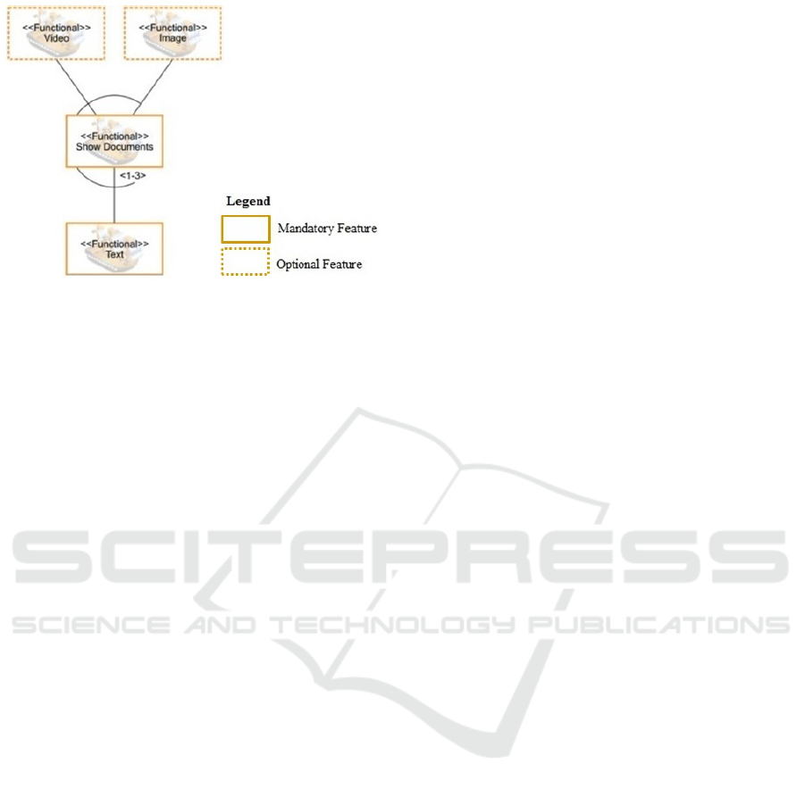
Figure 2: A variation point of the Mobile Guide feature mo-

del (Marinho et al., 2013).

charge level is high, all document types are available.

Low, medium and high values are deﬁned empirically

before the application is deployed.

As “Text” is a mandatory feature, it has to be al-

ways active. However, as regards to the other two

features of the variation point Show Documents, the

following question arises in the product conﬁguration

for the initial launch: Should we bind the features

“Video” and “Image” permanently at static binding

time or should we leave them to be bound dynami-

cally (at runtime) according to the changes in the bat-

tery charge level?. Thus, in our example, we have

four options: (i) only static binding for both features;

(ii) dynamic binding for both features; (iii) only static

binding for the feature “Video” and dynamic binding

for the feature “Image”; and (iv) only static binding

for the feature “Image” and dynamic binding for the

feature “Video”.

By applying only the static binding, we affect the

dynamicity of the product, but this can be necessary

to satisfy the resource constraints (e.g., time spent in

the activation/deactivation of features). Then, to ans-

wer the question aforementioned, we need feature at-

tributes related to the binding time to decide the best

option to satisfy both the customer and the resource

constraints. Depending on the attributes values, for a

given customer, for example, it can be more interes-

ting to remove the feature “Video” permanently (sta-

tic binding) and leave only the feature “Image” to be

bound at runtime (dynamic binding).

Therefore, the problem is to derive a partial pro-

duct conﬁguration from a DSPL, with the maximum

adaptability (the main goal of a DSPL), maximum va-

lue to the customer (to satisfy him/her), and minimum

cost (to optimize the resources), respecting the feature

model rules (to be a valid product).

4 A GRAPH MODEL

FORMULATION FOR FEATURE

SELECTION IN DSPL

In this section, we describe our graph model, the pro-

blem objectives of our formulation and the feasibility

rules.

4.1 A Graph Model

In our formulation, from the feature model, we gene-

rate a directed graph for the veriﬁcation of the rules of

this model and the identiﬁcation of feasible solutions

to the feature selection problem in a DSPL.

The graph G = (V, E) represents the features and

the relationships between features deﬁned by feature

model rules. Each vertex x ∈ V corresponds to a fe-

ature of the model. The vertices are divided into two

sets that indicate if the feature is optional or manda-

tory.

V = V

∪V

where

V m =



x ∈ V

|x is a mandatory feature}

Vo =



x ∈ V

|x is a optional feature}

In order to deﬁne the graph edges, three concepts

are used: feature dependency, feature proximity, and

statically exclusion. When a feature x depends on a

feature y, it means that the feature x requires y. The

proximity of a feature x is the set of features so that

x requires at least one of the features in its proximity.

If a feature x excludes statically a feature y, then both

x and y cannot be activated simultaneously in the pro-

duct.

Thus, the set of edges E is divided into three sub-

sets, where each subset denotes an edge type.

E = E

∪ Ev ∪ E

where

Ed =



xy ∈ E

|x depends on y}

Ev =



xy ∈ E

|y belongs to the proximity of x}

Ee =



xy ∈ E

|x excludes statically y}

Table 1 shows how the vertices and edges are re-

presented in the graph. Mandatory features (set V

)

generate ﬁlled vertices. Optional features (set V

) ge-

nerate unﬁlled vertices. Edges from the set E

are

represented by continuous arcs. Edges from the set

are represented by dotted arcs. Lastly, edges from

the set E

are represented by dashed arcs.

ICEIS 2018 - 20th International Conference on Enterprise Information Systems

148

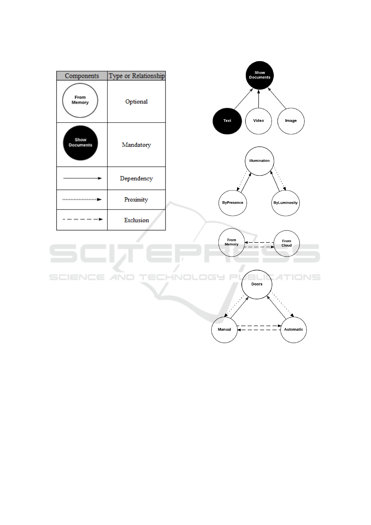
Table 1: Graph Components.

A feature model may have also a set of fea-

ture groups (FG). Each group g has a minimum

(minFG(g)) and maximum (maxFG(g)) quantity of

features that may be active at the same time in the pro-

duct. In the graph, there are no speciﬁc components

to represent the feature groups, but they can be added

during the implementation of the graph data structure,

as exempliﬁed in our proof of concept (see Section 5).

Figure 3 shows the relationships among the fea-

tures in the graph. Figure 3.a shows an example of

father and son relationship. In this ﬁgure, the features

“Text”, “Video” and “Image” can only be selected, if

“Show Documents” was selected. In Figure 3.b, an

example of require relationship with the operator Or

is presented. In this case, if the feature “Illumination”

is selected, it requires that at least one feature from

the set [“ByPresence”, “ByLuminosity”] is selected.

Figure 3.c shows an exclude relationship, where

if a feature in this relationship is activated, the other

cannot be activated at the same time. Then, if a fe-

ature is related to others by dashed edges, and this

feature is selected for the product as static, the others

cannot be selected to the product. Lastly, Figure 3.d

shows a require relationship using the operator Xor.

In the latter, if the feature “Doors” is selected, it re-

quires that at least one among the features “Manual”

and “Automatic” is selected. Moreover, if a feature

among the features “Manual” and “Automatic” is se-

lected at static time to be always active, the other fea-

ture cannot be selected.

(a) father and son dependence

(b) require with the operator Or

(d) require with the operator Xor

Figure 3: Feature model relationships represented in the

graph.

4.2 Problem Objectives

In our problem formulation, presented bellow, a so-

lution F

is composed by a subset of features of the

feature model selected for the product. The dynami-

city of the DSPL products can be improved by maxi-

mizing the number of features with dynamic binding

(1). Moreover, to better satisfy the user, we should

maximize the value (value( f

)) (2) of the features se-

lected ( f

), which can be measured through feature

Optimized Feature Selection for Initial Launch in Dynamic Software Product Lines

149

attributes like utility or quality attributes (even those

related to the context awareness). Despite limiting the

feasible solutions to a resource constraint, we suggest

to use an objective to minimize the cost (cost( f

)) of

the features (3). This cost can be, for example, regar-

ding performance, resource usage, or monetary value.

Thus, the results of the optimization process with a

multi-objective algorithm show a set of options with

different costs that the customer may choose. As we

discussed in the previous sections, since the DSPL fe-

atures can be bound statically or dynamically, we con-

sider two kinds of costs: i) CostD, which is the feature

cost when it is left to the dynamic bind; and ii) CostE,

which is the feature cost when it is bound only stati-

cally.

Maximize

∑

∈F

dynamicity( f

) (1)

Maximize

∑

∈F

value( f

) (2)

Minimize

∑

∈F

cost( f

) (3)

where

dynamicity( f

) =











1, if f

is selected with

bound dynamically

0, if f

is selected with

bound only statically

cost( f

) =



costD, if dynamicity( f

) = 1

costE, if dynamicity( f

) = 0

4.3 Feasibility Rules

In our formulation, a solution is feasible only if it re-

spects the following constraint:

brokenFeasibilityRules(F

) = 0 (4)

It means that all feasibility rules, i.e., the feature

model rules (see Section 4.3.2), should be satisﬁed by

the solution.

4.3.1 Vertex Value

Each vertex x, related to a feature, has an integer s(x),

that indicates the state of the feature. The possible

values to s(x) are:

s(x) =







0, if feature x was not selected

1, if feature x was selected as static

2, if feature x was selected as dynamic

We can also deﬁne num

(g) and num

(g) as the

number of features in a group g selected as static

and dynamic, respectively. Then, num

(g) =|{x ∈ g |

s(x) = 1}| and num

(g) =|{x ∈ g | s(x) = 2}|.

4.3.2 Rules

A solution is feasible if the following rules are satis-

ﬁed:

1. If x ∈ V

, then s(x) = 1

• If the feature is mandatory, it must be selected

at static time;

2. If x,y ∈ V and xy ∈ E

, then if s(x) 6= 0, then

s(y) 6= 0

• If a feature x depends on a feature y, feature x

can just be selected if y is also selected;

3. If x ∈ V and Y ⊂ V, such that Y = {y ∈ Y | y 6= x

and xy ∈ E

}, then if s(x) 6= 0, then

∑

y∈Y

s(y) > 0

• If a set of features Y belongs to the proximity of

a feature x, then feature x can only be selected,

if at least one of the features in set Y is also

selected;

4. If x, y ∈ V and xy ∈ Ee, then if s(x) = 1, then

s(y) = 0

• If a feature x excludes a feature y, and the fea-

ture x is selected as static, then feature y cannot

be selected;

5. ∀g ∈ FG,

∑

num

(g) ≤ maxFG(g)

• The solution cannot select more static features

belonging to the same group than the maximum

number of active features allowed at the same

time in that group;

6. ∀g ∈ FG,

∑

num

(g)) +

∑

num

(g) ≥ minFG(g)

• The number of selected features belonging to

a group, independently of if static or dynamic,

must be greater than or equal to the minimum

number of features that may be active at the

same time in that feature group;

∑

∈F

cost( f

) ≤ maxCost

• The cost of the solution should be less than

maxCost, which is a maximum cost that the cu-

stomer is willing to spend;

Rule 1 is used to check if the feature is mandatory.

Rules 2 to 4 validate the relations depicted in Figure 3.

Rules 5 and 6 are used to validate the feature groups

rules. Lastly, rule 7 limits the cost of the product.

ICEIS 2018 - 20th International Conference on Enterprise Information Systems

150

5 PROOF OF CONCEPT

A proof of concept was performed to verify the fea-

sibility of using the graph model and the formulation

proposed for solving the feature selection problem in

a DSPL. In our proof of concept, we used three fe-

ature models: (i) Mobiline, discussed in Section 3.1;

(ii) a DSPL for smart homes, called SmartHome (Car-

valho et al., 2017); and (iii) one artiﬁcially generated

feature model.

We used the framework JMetal (Durillo and Ne-

bro, 2011) to run the proof of concept with the algo-

rithm NSGAII (Deb et al., 2002a) and IBEA (Sayyad

et al., 2013b). These algorithms were selected, be-

cause they are used in several related work that deal

with feature selection (Pascual et al., 2013a)(Sayyad

et al., 2013a).

5.1 Population Representation

We represent a DSPL feature model with “n” features

through two strings S1 and S2 of “n” binary digits. In

S1, the value “1” for a digit indicates that the feature

is selected (“0” for unselected feature). In S2, the va-

lue “1” for a digit indicates that the feature should be

bound dynamically, while “0” means that the feature

should be bound only statically. For example, Table

2 shows the representation of two products with both

strings S1 and S2. In Product 1, the feature “Video”

was not selected (its corresponding bit in S1 = 0), and,

in this case, it does not matter its value in S2 (could be

0 or 1). Besides, in Product 1, the feature “Image” is

selected, but at the static binding time (its correspon-

ding bit in S2 = 0), meaning that it is always active.

In Product 2, both features “Image” and “Video” are

selected (bit in S1 = 1) and left to be bound at runtime

(bit in S2 = 1).

Table 2: Example of product representation.

Product Feature bit of S1 bit of S2

Product 1

Image 1 0

Video 0 0/1

Product 2

Image 1 1

Video 1 1

In relation to the features states presented in

Section 4.3.1, when the value s(x), associated to the

feature represented by the vertex x in the graph, is 0,

it means that S1 = 0. When S1 = 1 and S2 = 0, we

have s(x) = 1. And when S1 = 1 and S2 = 1, we have

s(x) = 2.

5.1.1 Feature Models Setting

Henceforward, we call the feature model from the

Mobiline project (Marinho et al., 2013) as Mob, the

model of SmartHome as Sma, and the artiﬁcial fea-

ture model as 200D. To generate the artiﬁcial DSPL

feature model, we used a procedure based on the met-

hod of Thum et al. (Thum et al., 2009) to randomly

create a feature model.

Table 3 presents an overview of the feature models

used in the experiments. In this table, we show the

number of features and rules of the models used.

Table 3: Feature models used in the experiment.

Model N. of features N. rules

Mob 33 24

Sma 17 19

200D 200 128

5.1.2 Feature Values and Costs

The value of a feature indicates their relevance to the

customer and can be deﬁned by the Requirement Ana-

lyst according to the requirements provided by the cu-

stomer. In our proof of concept, we consider that the

value of a feature can vary from 0 to 5 according to

their level of relevance to the customer, where:

value =











0, if the feature is irrelevant

1, if the feature is very little relevant

2, if the feature is somewhat relevant

3, if the feature is moderately relevant

4, if the feature is very relevant

5, if the feature is extremely relevant

In an SPL or DSPL, the cost of a feature must be

deﬁned by the development team, because it is rela-

ted to the cost of generating and modifying the assets

(e.g., code elements) which will compose the featu-

res (Cruz et al., 2013) (Santos Neto et al., 2016). We

suggest the following formulas to calculate the costs

of the feature in static (costE) and dynamic (costD)

binding:

costE = costIN + costBA + costCF and

costD = costIN + costBA + costCF + costAD

where

• costIN is the inherent cost of using the feature,

which includes the value of use of the feature and

its assets that were created during the DSPL engi-

neering process;

• costBA is the average cost of energy consumption

of the feature in the deploy environment;

• costCF is the cost of customizing feature assets

for the product;

• costAD is the cost of the insertion of the runtime

adaptation logic; this cost is related to the context-

awareness of DSPLs;

Optimized Feature Selection for Initial Launch in Dynamic Software Product Lines

151

We also consider that each of these costs can as-

sume a value between 0 and 5 according to the level

of complexity of the task associated (costIN, costCF,

costAD) or energy consumption (costBA), where:

cost =











0, if it does not exists

1, if it is too low

2, if it is low

3, if it is moderate

4, if it is high

5, if it is too high

The level of complexity, mentioned before, invol-

ves not only the difﬁculty of carrying out the task but

also the time spent on it and the impact on the product.

The values and costs for Mobiline and Smart-

Home models were generated artiﬁcially following

the above-mentioned ranges. To obtain the real costs,

it is needed to survey the customers and developers of

this DSPLs, but this was out of the scope of this work.

For the artiﬁcial DSPL, the costs and values were also

generated randomly.

5.1.3 Setting Up the Algorithm

In the algorithms used in the proof of concept, we ap-

plied the following parameters: Population Size of

100, Crossover (Single-Point Crossover) Probability

of 0.9 and Mutation (Bit-Flip Mutation) Probability

of 0.05. Besides, for the feature models (Mob, Sma,

200D), we ran the algorithms with 200k evaluations.

In all cases, each algorithm run was repeated 30 times

for ensuring more reliability.

5.1.4 The Graph

In our proof of concept, the graph is represented as

an object. Besides, we use the adjacent list concept

for its representation. In practice, a vector of Vertex

objects was created, where each Vertex contains a

list of edges, which have this vertex as origin, and a

color (black or white), to verify whether the feature

related to the vertex is mandatory or not. Each edge is

represented by a tuple that indicates the destiny vertex

of the edge and a type (continuous, dotted or dashed),

to denote to which set of edges (see Section 4.1) it

belongs. Lastly, the GraphModel object also has a

second list containing the features groups.

5.2 Execution Flow

Figure 4 shows the ﬂowchart of the execution of our

proof of concept. The process started when the fea-

ture model was used as input to our ﬂow. Next, the

Figure 4: Proof of Concept ﬂowchart.

graph is generated, and the multi-objective optimiza-

tion algorithm was conﬁgured. Once the conﬁgurati-

ons are done, we executed the optimization algorithm.

During the execution of each loop of the optimization

algorithm, the graph was used to validate solutions.

At the end of the execution of the algorithm, the

best valid solutions were identiﬁed. We can consider

the best solutions like the one with the highest dyna-

micity, the lowest cost, the best value, or those soluti-

ons that are closest to the Pareto front, such as, we can

use measures like SPREAD (Deb et al., 2002b) and

Hypervolume (HV) (Zitzler and Thiele, 1999). Table

4 presents the average of the number of correct solu-

tions, solution values, solution costs, number of dyn-

amic features, HV and SPREAD. These values were

generated by the optimization algorithms using Mob,

Sma and 200D models considering a maximum cost

equals to 400 for the ﬁrst two models and 700 for the

last one. Table 5 presents three feasible solutions for

SMA model after running the optimization algorithm

NSGAII. This data can be used to assistant the choose

of the most appropriate solution for the product of the

DSPL.

Lastly, the DSPL Requirement Analyst selects the

solution from which a feature model will be gene-

rated to be used by the development team. In our

proof of concept, for each valid solution selected,

an XML ﬁle following a pattern similar to the one

used by the Software Product Line Online Tools

(S.P.L.O.T)(Mendonca et al., 2009) can be generated

as output. Figure 5 presents an example of the gene-

rated XML ﬁle, and the corresponding features, from

the Solution 1 presented in Table 5.

5.3 Discussion

This proof of concept shows initial evidence that

our model can be used to provide an optimized way

to solve the feature selection problem for the initial

launch in DSPL. Our model allows the use of dif-

ferent optimization algorithms to check and generate

optimal solutions.

Regarding Table 4, it is possible to verify a large

ICEIS 2018 - 20th International Conference on Enterprise Information Systems

152

Table 4: Results of the executions of the optimization algorithms.

Alg Mod Correctness Value Cost D. Feat. SPREAD HV

NSGA

Mob 34.86 ± 3.7 52 ± 1.7 290.49 ± 8.34 14.5 ± 0.5 0.70 ± 0.03 0.41 ± 0.004

Sma 50.16 ± 2.0 59 ± 0.6 173.42 ± 2.18 4.5 ± 0.5 0.91 ± 0.03 0.40 ± 0.002

200D 18 ± 6.4 233 ± 17 497.40 ± 41.87 28.5 ± 3.5 0.66 ± 0.04 0.34 ± 0.008

IBEA

Mob 2.6 ± 1.47 64.4 ± 1.8 375.05 ± 10.88 22.23 ± 0.6 0.64 ± 0.02 0.47 ± 0.003

Sma 44.3 ± 1.23 62.6 ± 0.1 196.82 ± 0.91 7 ± 0 0.97 ± 0.02 0.42 ± 0.001

200D 65.5 ± 6.1 307.7 ± 6.5 557.18 ± 13.31 40.7 ± 1.5 0.57 ± 0.03 0.47 ± 0.007

Table 5: Example of solutions for Smart Home (Sma) DSPL.

Variable 1 Variable 2 Value Cost D. Feat.

Solution 1 11111101011101010 00100100000101010 44.0 128.0 5

Solution 2 11111101011111010 00000000000101000 49.0 128.0 2

Solution 3 11111101011111010 00000100000100010 49.0 132.0 3

variation of the results obtained by the algorithms

used. This variation came from the implementation of

the algorithms. In a nutshell, it is possible to realize

that the NSGA algorithm generated on average soluti-

ons with lower costs, but the IBEA algorithm genera-

ted on average solutions with better values and more

dynamic features. We believe that the small number

of correct solutions generated by the IBEA algorithm

for the Mobiline features model is a result of the max-

imum cost that was overcome by the majority of the

solutions generated by the IBEA. In the other models,

this does not occur. In these models, it is possible

to note that the average cost was considerably lower

than the maximum cost established. Finally, the small

amount of correct solutions obtained by the NSGA

algorithm for the 200D model corroborates with what

was stated in (Sayyad et al., 2013b), that indicated the

NSGA algorithm tends to deteriorate rapidly.

We emphasize that the detailed comparison of the

results generated by the optimization algorithms goes

beyond the scope of this paper. Thus, it is important

to highlight that the goal of this proof of concept was

not to present the best solution regarding the model

implementation or the best optimization algorithm to

solve the problem of the selection of features in DS-

PLs.

In addition, the difﬁculty to obtain real Dyna-

mic Software Product Lines, as cited also in (Bezerra

et al., 2016), makes it difﬁcult to evaluate the optimi-

zation model for the feature selection problem in the

real environment. Lastly, the study of the best algo-

rithms to solve the presented problem is left as future

work.

5.4 Threats to Validity

One threat to the validity of the results is the use of

synthetic data as attributes of features, i.e., values,

cost and the DSPL generated artiﬁcially. We produce

these data artiﬁcially due to the difﬁculty of obtaining

real DSPL data. The generation of synthetic data has

also been used by other authors in experiments with

search-based algorithms (Sayyad et al., 2013b)(Guo

et al., 2011).

It is important to emphasize that there is not a pre-

cise way to deﬁne the feature cost since it depends

on the implementation of the product. In (Cruz et al.,

2013) and (Santos Neto et al., 2016) are presented es-

timation approaches for generating this cost, but this

forecast depends on the information of the assets rela-

ted to each feature, and measures correlated to them.

For example, these approaches use the number of li-

nes of code and coupling of an asset.

Another threat to validity is related to the Pareto

Front generated from the JMetal (i.e., without using

a brute force search algorithm to ﬁnd the real Pareto

Front). This can have impacted the results of the eva-

luations, because it may not be the best solution. Be-

sides, the way with the structure of the graph was im-

plemented affects both time and correctness rate and,

therefore, more experiments are required to measure

the impact of this implementation on the objectives

optimized.

6 RELATED WORK

We identiﬁed in the literature related work to the

feature selection problem in a SPL (Guo et al.,

2011)(lin Wang and wei Pang, 2014)(Sayyad et al.,

2013b)(Henard et al., 2015) and in a DSPL (Pas-

cual et al., 2013b; Pascual et al., 2015)(Pascual et al.,

2013a)(Sanchez et al., 2013).

Guo et al. (Guo et al., 2011) and Wang and Pang

(lin Wang and wei Pang, 2014) present approaches

mono-objective for SPL feature selection. Guo et al.

(Guo et al., 2011) use Genetic Algorithm to ﬁnd an

optimized feature selection that minimizes or max-

Optimized Feature Selection for Initial Launch in Dynamic Software Product Lines

153

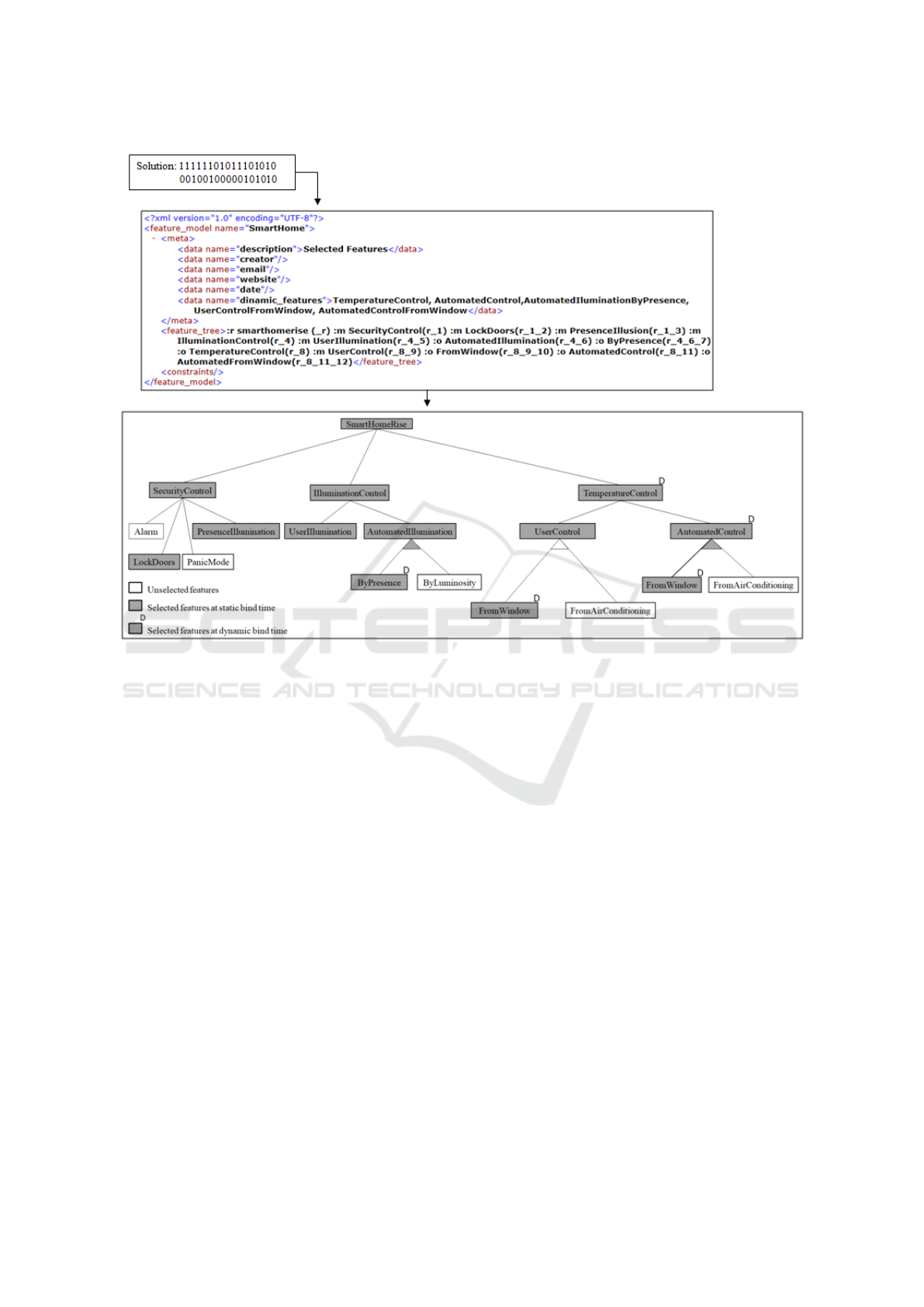
Figure 5: Example of solution for the SmartHome DSPL.

imizes an objective function. Wang and Pang (lin

Wang and wei Pang, 2014) uses a graph to represent

a feature model and an ant colony optimization to get

a solution to the SPL feature selection optimization

problem that maximizes the product value subject to

constraints.

Sayyad et al. (Sayyad et al., 2013b) compare the

results of seven multi-objective evolutionary optimi-

zation algorithms using up to ﬁve optimization ob-

jectives. Christopher et al. (Henard et al., 2015) pro-

pose SATIBEA, an approach for conﬁguring massive

SPLs with over ﬁve thousand features using an appro-

ach that blends an optimization by merging the IBEA

algorithm and a model validation using SAT solver.

In the DSPL scenario, Pascual et al. (Pascual

et al., 2013b; Pascual et al., 2013a; Pascual et al.,

2015) describe an approach for the automatic runtime

generation of application conﬁgurations and reconﬁ-

guration plans in a DSPL. The goal of this approach

is to choose the architectural conﬁguration, using a

genetic algorithm, which provides the best functiona-

lity, while not exceeding the available resources (e.g.,

memory) at runtime. Sanchez et al. (Sanchez et al.,

2013) propose an algorithm for selecting at runtime

the conﬁguration that optimizes given quality metrics.

The goal of this approach is to determine the arrange-

ment most suitable, especially concerning the follo-

wing non-functional aspects: quality of service, per-

formance, and reconﬁguration time.

As described in the previous paragraphs, we iden-

tiﬁed work related to the feature selection problem

in SPL (Guo et al., 2011)(Wang and Peng, 2014)

(Sayyad et al., 2013b) (Henard et al., 2015) and some

work dealing with the feature selection problem in

a DSPL at runtime (Pascual et al., 2013b) (Pascual

et al., 2013a) (Pascual et al., 2015) (Sanchez et al.,

2013).

The studies focused on SPL do not address run-

time adaptation, and then, they do not take into ac-

count the dynamic binding time. The latter, addres-

sing DSPLs, were worried with the optimization of

the resources used (Pascual et al., 2013a)(Pascual

et al., 2013b)(Pascual et al., 2015) or of quality me-

trics at runtime (Sanchez et al., 2013). Thus, these

studies do not support the decision of which features

should be bound statically and which one should be

bound dynamically.

We also ﬁnd in the literature related work (White

ICEIS 2018 - 20th International Conference on Enterprise Information Systems

154

et al., 2014) (Lochau et al., 2017) that considers

the multi-step conﬁguration problem to DSPL, that

involves transitioning from a starting conﬁguration

through a series of intermediate conﬁgurations to a

conﬁguration that meets a desired set of end state re-

quirements. However, these studies do not aim to

achieve a feature optimized conﬁguration. Thus, the

difference of our work is that our proposed graph mo-

del can solve the feature selection problem in DSPL’s

by indicating a optium solution and considering both

the static and dynamic binding time.

7 CONCLUSIONS

In a typical SPL, the feature selection is made stati-

cally only, whereas in a DSPL we also have the dyna-

mic binding to provide product adaptation at runtime.

This runtime adaptation introduces a cost that can be

reduced by deﬁning a partial product conﬁguration for

initial launch.

We proposed a graph model and a multi-objective

formulation that considers both static and dynamic

binding time to help in the decision of which features

should be bound permanently at static binding time

and which features should be bound at the dynamic

binding time. Our model allows the use of different

techniques to check and generate the optimal soluti-

ons.

We also presented a proof of concept that shows

the feasibility of using our model to obtain optimized

feature model conﬁgurations, indicating if the featu-

res should have to be bound at the static or dynamic

time. With this information, the Requirement Analyst

has a set of feasible submodels (i.e., DSPL products)

to be offered to the customer.

As future work, it can be veriﬁed other ways to

implement the graph structure and the best way to cal-

culate the cost of dynamic feature (costD) and static

feature (costE). Also, experiments can be performed

to assess what is the best multi-objective optimization

algorithm to be used for our proposed formulation.

Moreover, it would be interesting to investigate if the

proposed graph could be adapted to check a feasibi-

lity of the features model at runtime when there is a

change in the product.

REFERENCES

Benavides, D., Segura, S., and Ruiz-Cort

es, A. (2010). Au-

tomated analysis of feature models 20 years later: A

literature review. Inf. Syst., 35(6):615–636.

Bencomo, N., Hallsteinsen, S., and Santana de Almeida, E.

(2012). A view of the dynamic software product line

landscape. Computer, 45(10):36–41.

Bezerra, C. I., Andrade, R. M., and Monteiro, J. M. (2016).

Exploring quality measures for the evaluation of fe-

ature models: a case study. Journal of Systems and

Software.

Capilla, R., Bosch, J., Trinidad, P., Cort

es, A. R., and Hin-

chey, M. (2014). An overview of dynamic software

product line architectures and techniques: Observati-

ons from research and industry. Journal of Systems

and Software, 91:3–23.

Carvalho, M. L. L., da Silva, M. L. G., da Silva Gomes,

G. S., Santos, A. R., do Carmo Machado, I., de Je-

sus Souza, M. L., and de Almeida, E. S. (2017). On

the implementation of dynamic software product li-

nes: An exploratory study. Journal of Systems and

Software, 136(Supplement C):74 – 100.

Chakravarthy, V., Regehr, J., and Eide, E. (2008). Edicts:

Implementing features with ﬂexible binding times. In

Proceedings of the 7th International Conference on

Aspect-oriented Software Development, AOSD ’08,

pages 108–119, New York, NY, USA. ACM.

Cruz, J., Neto, P. S., Britto, R., Rabelo, R., Ayala, W., Soa-

res, T., and Mota, M. (2013). Toward a hybrid appro-

ach to generate software product line portfolios. In

Evolutionary Computation (CEC), 2013 IEEE Con-

gress on, pages 2229–2236. IEEE.

Deb, K., Pratap, A., Agarwal, S., and Meyarivan, T.

(2002a). A fast and elitist multiobjective genetic al-

gorithm: Nsga-ii. IEEE transactions on evolutionary

computation, 6(2):182–197.

Deb, K., Pratap, A., Agarwal, S., and Meyarivan, T.

(2002b). A fast and elitist multiobjective genetic al-

gorithm: Nsga-ii. Evolutionary Computation, IEEE

Transactions on, 6(2):182–197.

Durillo, J. J. and Nebro, A. J. (2011). jMetal: A java fra-

mework for multi-objective optimization. Advances in

Engineering Software, 42:760–771.

Eriksson, M. and Hagglunds, A. (2003). An introduction

to software product line development. In Proceedings

of Ume

a’s Seventh Student Conference in Computing

Science, UMINF, volume 3, pages 26–37.

Fernandes, P., Werner, C., and Teixeira, E. (2011). An

approach for feature modeling of context-aware soft-

ware product line. The Journal of Universal Computer

Science, 17(5).

Guo, J., White, J., Wang, G., Li, J., and Wang, Y. (2011). A

genetic algorithm for optimized feature selection with

resource constraints in software product lines. J. Syst.

Softw., 84(12):2208–2221.

Hallsteinsen, S., Hinchey, M., Park, S., and Schmid, K.

(2008). Dynamic software product lines. Computer,

41(4):93–95.

Harman, M., Jia, Y., Krinke, J., Langdon, W. B., Petke, J.,

and Zhang, Y. (2014). Search based software engi-

neering for software product line engineering: A sur-

vey and directions for future work. In Proceedings of

the 18th International Software Product Line Confe-

Optimized Feature Selection for Initial Launch in Dynamic Software Product Lines

155

rence - Volume 1, SPLC ’14, New York, NY, USA.

ACM.

Henard, C., Papadakis, M., Harman, M., and Le Traon,

Y. (2015). Combining multi-objective search and

constraint solving for conﬁguring large software pro-

duct lines. In Software Engineering (ICSE), 2015

IEEE/ACM 37th IEEE International Conference on,

volume 1, pages 517–528. IEEE.

Kang, K. C., Cohen, S. G., Hess, J. A., Novak, W. E.,

and Peterson, A. S. (1990). Feature-oriented dom-

ain analysis (foda) feasibility study. Technical report,

Carnegie-Mellon Univ Pittsburgh Pa Software Engi-

neering Inst.

lin Wang, Y. and wei Pang, J. (2014). Ant colony optimi-

zation for feature selection in software product lines.

Journal of Shanghai Jiaotong University (Science),

19(1):50–58.

Lochau, M., B

urdek, J., H

olzle, S., and Sch

urr, A. (2017).

Speciﬁcation and automated validation of staged re-

conﬁguration processes for dynamic software product

lines. Software & Systems Modeling, 16(1):125–152.

Lopez-Herrejon, R. E., Linsbauer, L., and Egyed, A. (2015).

A systematic mapping study of search-based software

engineering for software product lines. Information

and Software Technology, 62:33–51.

Marinho, F. G., Andrade, R. M. C., Werner, C., Viana, W.,

Maia, M. E. F., Rocha, L. S., Teixeira, E., Filho, J. a.

B. F., Dantas, V. L. L., Lima, F., and Aguiar, S. (2013).

Mobiline: A nested software product line for the dom-

ain of mobile and context-aware applications. Sci.

Comput. Program., 78(12):2381–2398.

Mendonca, M., Branco, M., and Cowan, D. (2009). Splot:

software product lines online tools. In Proceedings

of the 24th ACM SIGPLAN conference companion on

Object oriented programming systems languages and

applications, pages 761–762. ACM.

Olaechea, R., Rayside, D., Guo, J., and Czarnecki, K.

(2014). Comparison of exact and approximate multi-

objective optimization for software product lines. In

Proceedings of the 18th International Software Pro-

duct Line Conference - Volume 1, pages 92–101, NY,

USA. ACM.

Pascual, G. G., Lopez-Herrejon, R. E., Pinto, M., Fuentes,

L., and Egyed, A. (2015). Applying multiobjective

evolutionary algorithms to dynamic software product

lines for reconﬁguring mobile applications. Journal of

Systems and Software, 103:392–411.

Pascual, G. G., Pinto, M., and Fuentes, L. (2013a). Run-

time adaptation of mobile applications using genetic

algorithms. In Proceedings of the 8th International

Symposium on Software Engineering for Adaptive and

Self-Managing Systems, pages 73–82, Piscataway, NJ,

USA. IEEE Press.

Pascual, G. G., Pinto, M., and Fuentes, L. (2013b). Run-

time support to manage architectural variability spe-

ciﬁed with cvl. In Proceedings of the 7th European

Conference on Software Architecture, ECSA’13, pa-

ges 282–298, Berlin, Heidelberg. Springer-Verlag.

Rosenm

uller, M., Siegmund, N., Apel, S., and Saake, G.

(2011). Flexible feature binding in software product

lines. Automated Software Engg., 18(2):163–197.

Rosenm

uller, M., Siegmund, N., Saake, G., and Apel, S.

(2009). Combining static and dynamic feature binding

in software product lines. Technical report ﬁn-013,

Otto-von-Guericke-Universit at Magdeburg.

Sanchez, L. E., Moisan, S., and Rigault, J.-P. (2013).

Metrics on feature models to optimize conﬁguration

adaptation at run time. In Proceedings of the 1st In-

ternational Workshop on Combining Modelling and

Search-Based Software Engineering, pages 39–44,

NJ, USA. IEEE Press.

Santos Neto, P. d. A., Britto, R., Rab

elo, R. d. A. L., de Al-

meida Cruz, J. J., and Lira, W. A. L. (2016). A hybrid

approach to suggest software product line portfolios.

Applied Soft Computing, 49:1243–1255.

Sayyad, A. S., Ingram, J., Menzies, T., and Ammar, H.

(2013a). Optimum feature selection in software pro-

duct lines: Let your model and values guide your

search. In Proceedings of the 1st International

Workshop on Combining Modelling and Search-Based

Software Engineering, pages 22–27, Piscataway, NJ,

USA. IEEE Press.

Sayyad, A. S., Menzies, T., and Ammar, H. (2013b). On

the value of user preferences in search-based software

engineering: A case study in software product lines.

In Proceedings of the 2013 International Conference

on Software Engineering, pages 492–501, NJ, USA.

IEEE Press.

Thum, T., Batory, D., and Kastner, C. (2009). Reaso-

ning about edits to feature models. In Proceedings of

the 31st International Conference on Software Engi-

neering, ICSE ’09, pages 254–264, Washington, DC,

USA. IEEE Computer Society.

White, J., Galindo, J. A., Saxena, T., Dougherty, B., Benavi-

des, D., and Schmidt, D. C. (2014). Evolving feature

model conﬁgurations in software product lines. Jour-

nal of Systems and Software, 87:119–136.

Zitzler, E. and Thiele, L. (1999). Multiobjective evoluti-

onary algorithms: a comparative case study and the

strength pareto approach. IEEE Transactions on Evo-

lutionary Computation, 3(4):257–271.

ICEIS 2018 - 20th International Conference on Enterprise Information Systems

156