Concept for Intra-Hour PV Generation Forecast based on

Distributed PV Inverter Data

An Approach Considering Machine Learning Techniques and Distributed Data

Stefan Übermasser

, Simon Kloibhofer

, Philipp Weihs

and Matthias Stifter

AIT Austrina Institute of Technology, Giefinggasse 2, 1210 Vienna, Austria

Institute of Meteorology, University of Natural Resources and Life Sciences,

Gregor-Mendel-Straße 33, 1180 Vienna, Austria

Keywords: Distributed Data, Machine Learning, Photovoltaic Systems, Recurrent Neural Network, Power Forecast,

Short-Term Forecast, Renewable Energy, Distributed Energy Resources.

Abstract: The mass-introduction of small scale power generation units like photovoltaic systems at household levels

increase the risk for system unbalances, due to their stochastic generation profile. Additionally, upcoming

technologies such as electric vehicles, battery storage systems and energy management systems lead to a

change from consumer households to prosumers with a significant different residual load profile. For

optimizing the profile of future prosumers, especially the forecast for PV generation is crucial. Whilst

traditional weather forecasts are based on a few hundred metering locations in the case of Austria, more than

55000 PV systems are currently connected to the Austrian Power grid. Due to the low areal coverage of

common metering locations, weather forecasts do not take local phenomena like shadows from clouds into

account. An approach using generation data from neighbouring PV systems together with machine learning

methods provides a promising alternative for individual location based intra-hour forecasts. This paper

describes the requirements and methods of such a concept and concludes with a first proof of concept.

1 INTRODUCTION

The increasing introduction of distributed energy

resources (DER) like photovoltaic systems (PV) to

medium and low voltage distribution grids creates

new challenges but also chances for relevant

stakeholders like distribution system operators,

energy or service providers but also end customers.

Especially the fluctuating generation from PV

systems and the difficulties in forecasting changes in

power generation are causing increasing risks and

also costs in respect to a stable and reliable energy

supply and grid operation. Since a large share of PV

systems is installed directly at customer (prosumer)

premises, strategies for optimization at end customer

levels via home energy management systems

(HEMS) rely on as precise as possible intraday or

short-term forecasts for operating connected devices

(e.g. electric car, battery storage system …) as cost

efficient as possible. Power generation from PV

systems is highly influenced by local conditions (e.g.

clouds, temperature, type and setup of the system).

Hence, forecasting needs to take local parameters into

account which are based on satellite images or

stationary metering systems. For metering the

relevant parameters, in Austria less than 300 local

metering points exist (“Meteorological Network —

ZAMG,” 2017), which cannot provide the data which

is needed for an individual and local power forecasts

for PVs (see Figure 1).

Figure 1: Meteorological network of ZAMG (“Meteoro-

logical Network — ZAMG,” 2017) which offers

meteorological data from more than 250 meteorological

stations situated in all climate regions and altitudes Austria-

wide.

286

Übermasser, S., Kloibhofer, S., Weihs, P. and Stifter, M.

Concept for Intra-Hour PV Generation Forecast based on Distributed PV Inverter Data.

DOI: 10.5220/0006775802860293

In Proceedings of the 7th International Conference on Smart Cities and Green ICT Systems (SMARTGREENS 2018), pages 286-293

ISBN: 978-989-758-292-9

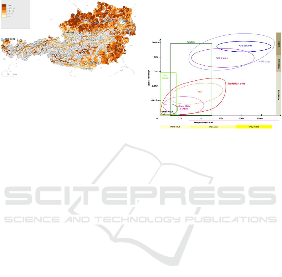
Figure 2: Distribution and number of PV systems in Austria

(systems per 1000 inhabitants) (“Photovoltaik Karten,”

2017).

In contrast there are currently more than 55.000

individual PV systems installed at the Austrian area

and counting. Those systems are spread out among all

populated areas of Austria (see Figure 2).

The growing numbers of high-resolution data

loggers (at inverters of PV systems) provide a high

potential for novel forecasting methods based on such

distributed measurements. Therefore, this approach is

taking into account spatial phenomena like cloud

movement. Using the individual generation data from

neighboring PV systems on machine learning

methods would enable approaches for local forecasts

for each PV site. In this paper a recurrent neural

network approach building on the open source

software library for machine intelligence

TensorFlow™ (“TensorFlow,” n.d.) is developed.

This approach is taking into account the spatial and

temporal dimension of power generation changes.

The goal is to show, that with this approach

significant improvements over forecasts based on

single site time series forecasts can be achieved.

State of the art forecasts for PV generation are

summarized in (Antonanzas et al., 2016). Most

popular are statistical methods relying on local

measurements for short forecast horizons and models

building on weather prediction for longer horizons

(see Figure 3). There are some approaches to include

also the data of neighbouring PV stations into the

forecast model. (Bessa et al., 2015) uses a vector

autoregressive (VAR) model to forecast 1 to 3 hours

ahead, showing improvement over an AR model

without other stations. (Lonij et al., 2013) uses a data

set of 80 rooftop PV systems on a 50x50 km area for

intra hour forecast. One of the problems occurring in

both references [5] and [6] are the coarse

measurement intervals of 15 minutes, which do not

allow following cloud shadows precisely.

Furthermore, there exist some larger scale projects,

like (Williamson, 2016), where a large number of

distributed sensors (PV inverters and fish eye cameras

for cloud detection) are connected with machine

learning techniques to improve the forecast over the

state of Canberra in Australia.

Figure 3: Overview of state of the art forecast methods for

PV generation (Antonanzas et al., 2016).

Machine learning techniques are already applied

in many publications of PV forecasting, but the

application is on a quite basic level up to now. Simple

feed-forward neural networks are used often, because

they are easily implemented, while advanced

architectures are not considered in literature. Areas

with advanced use of neural networks are for example

image recognition (e.g. for the detection of clouds and

wind direction or speed) and language processing.

While algorithms from image recognition cannot be

used for the concept described in this paper (because

they rely on strictly gridded spatial positions), the

time domain is represented very well in other areas of

research. Recurrent neural networks use the time

ordered nature of data for prediction. The long short-

term memory (LSTM) recurrent neural network for

example reaches outstanding scores at benchmarks

for speech recognition tasks (Graves et al., 2013).

Hence, the concept described in this work will use

recurrent neuronal networks.

The main focus of this paper is to describe the

general concept and the developed method and to

point out how a neural network method has to be

designed to fit this field, which differs in several

respects from classical machine learning disciplines.

First we apply a simplified scenario for a first proof

of concept. In future, special challenges including the

day cycle, irregularly spatial distribution of data

points, different weather regimes and other

parameters will be approached.

Concept for Intra-Hour PV Generation Forecast based on Distributed PV Inverter Data

287

2 CONCEPT DESCRIPTION

This position paper aims to describe a concept for an

intra-day PV generation forecast based on distributed

(neighbouring) PV generation data and machine

learning methods. The local generation from PV

Systems is influenced by a number of factors. In

general, the mathematical model for understanding

the PV generation profile can be divided into three

main models:

 Irradiation Model:

It describes the global radiation at a certain

location. Extra-terrestrial solar radiation can be

calculated based on geometric considerations.

Furthermore, the influence of the terrestrial

atmosphere on a clear day is often included into this

part of the model.

 Statistical Model:

This model describes the local disturbances

caused mainly by local weather phenomena.

 Physical Model:

The physical model contains the characteristics of

the technical system (cell type, inverter, position …).

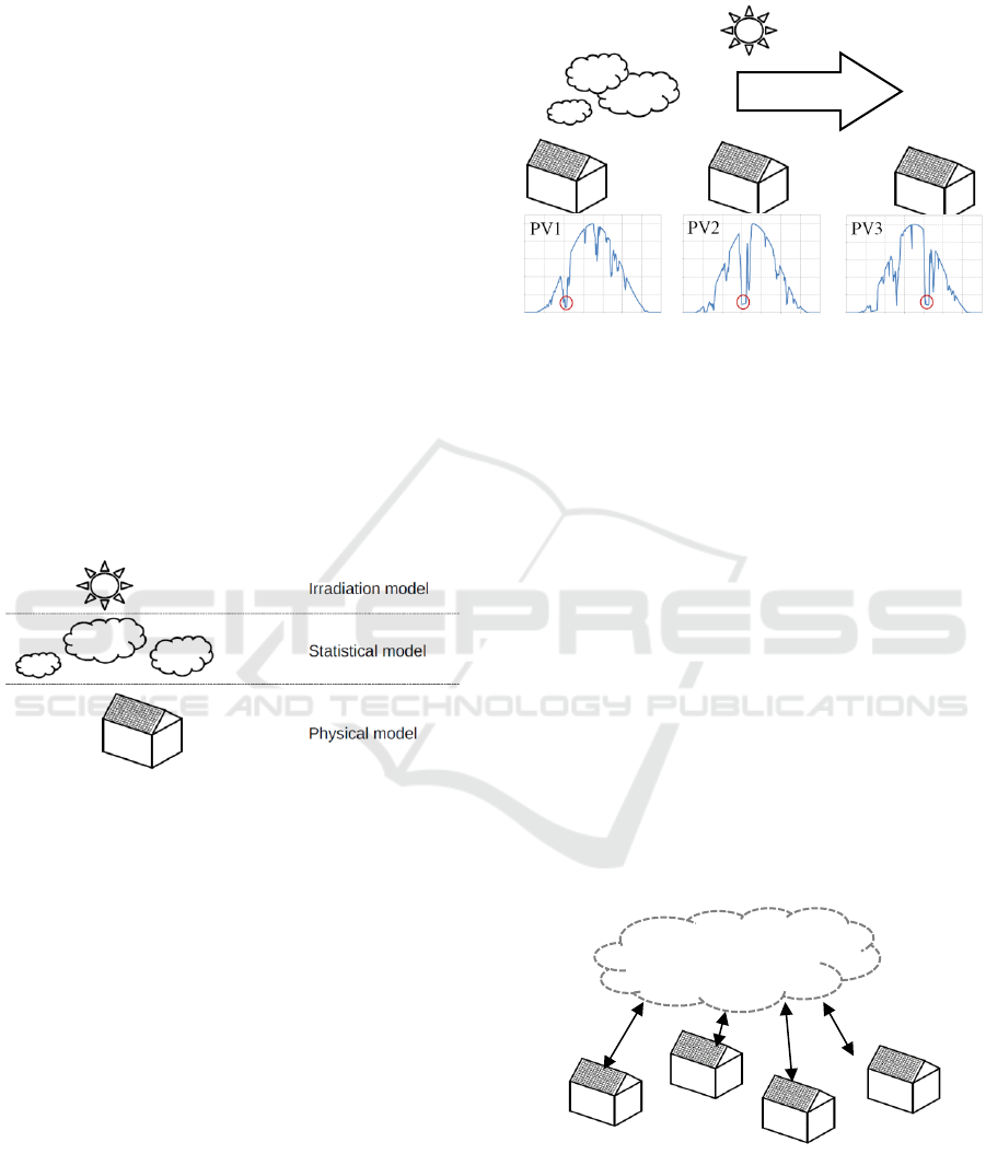
Figure 4: Types of models for the description of influence

parameters for PV generation and forecast.

Those three aspects are usually modelled

independently due to their diverse nature and

characteristics by different mathematical methods. In

reality, the effects of these three models are reflected

in the power generation profile of each PV system,

which can be measured directly at the inverter or grid

connection point. Whilst different mathematical

approaches were necessary in the past to conquer the

individual characteristics and challenges for each

model, progress in machine learning methods might

provide a new unified tool for the analysis of

generation data with respect to local power forecasts.

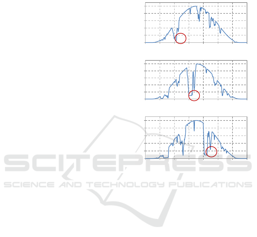
Figure 5 provides a schematic example of a time-

delayed power drop at neighboring PV systems

(along the wind direction) caused by a moving cloud.

Depending on the distance of the PV systems to each

other and the wind speed the probability for a similar

power drop at a neighboring PV system in direction

of the wind could be calculated.

Figure 5: Example of a time-delayed moving power drop at

neighbouring PV systems caused by a moving cloud (large

images of the PV diagrams in the APPENDIX).

As a requirement for the workability of the approach

described in this paper, participating PV Systems are

required to share the following data over a centralized

cloud based data infrastructure:

 Location [long/lat]: Geographical location of

the PV System. This information is necessary to

identify neighboring systems in reference to

wind direction and speed.

 Timestamp [yyyy-mm-dd hh:mm:ss]:

Timestamp of the data transmission consisting

of date and time. This information is necessary

to calculate forecasts.

 Power [kW]: The actual power output of the PV

system at a specific timestamp.

Such data needs to be submitted by each PV system.

This could either be done by a peer-to-peer network

or a centralized approach as shown in Figure 6.

Figure 6: Simplified data transfer between individual PV

systems by a centralized cloud system.

Wind direction

Data Cloud

SMARTGREENS 2018 - 7th International Conference on Smart Cities and Green ICT Systems

288

3 PROOF OF CONCEPT

Following the idea of the concept description (Section

2) basic requirements, method and a first use-case are

defined for a first proof of concept.

3.1 Requirement Analysis

In order to be able to establish a first proof of concept,

the requirements for method and use-case have to be

analysed. This section will mainly focus on the

requirements on data transmission and the

geographical distances between neighbouring

systems in dependence of wind speeds. As an

additional parameter, the forecasting horizon shall be

discussed to define the objective of this method.

Depending on the wind speed and the target

forecast horizon, the minimum distance to the next

neighboring system can be calculated. E.g. for a

forecast horizon of 15 minutes, the data signal of a

neighboring system would be needed 15 minutes

prior the forecasted point in time. This means

depending on the wind speed and assuming a real-

time signal transmission a minimum distance

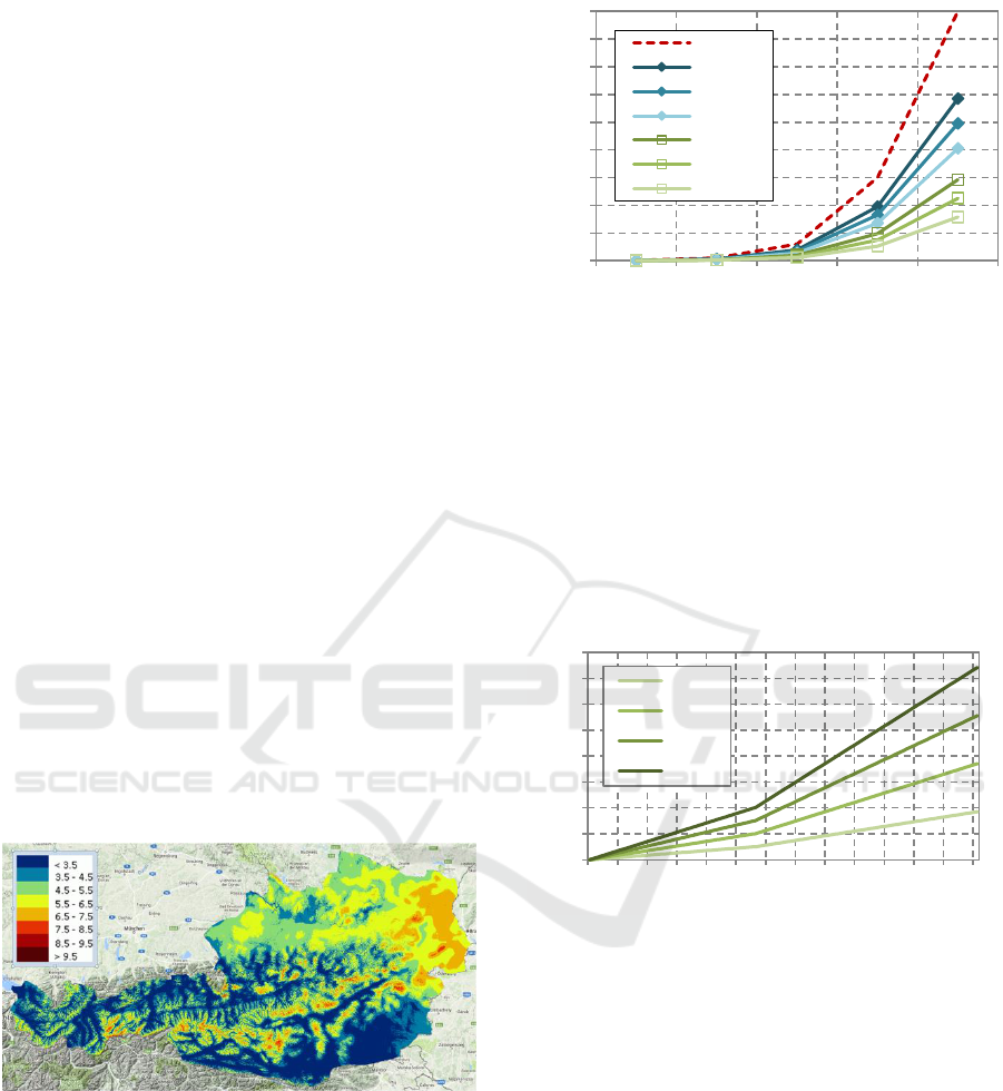
between sender and receiver is given. Figure 8 shows

the minimum distances between neighboring systems

for specific data transmission interval periods (from

one transmission per second down to every 900

seconds) in reference to wind speeds. According to

(“Windatlas Austria,” n.d.) average wind speeds at

100 meters above ground level are (depending on the

geographic area) between 4 and 7 m/s (see Figure 7).

Figure 7: Austrians geographical average annual wind

speed distribution (in m/s) (“Windatlas Austria,” n.d.).

Since clouds are situated above those heights, for

their movement higher wind speeds between 9 and 13

m/s must be considered (Lappalainen and

Valkealahti, 2016). From Figure 8 it can be followed

that data metering and the corresponding

transmission interval should be at least every 60

seconds, since slower intervals increase the distance

between systems significantly. This would enable the

Figure 8: Minimum distance of neighbouring systems

depending on data intervals and different wind speeds (4 to

20 m/s).

usage of signals from neighbouring systems of 1 km

distance. Even shorter transmission intervals would

be beneficial for increasing the forecasting quality

and for engaging shorter forecasting horizons (< 15

minutes). The higher the wind speed the more

distance is required between sender and receiver.

Figure 9 shows the minimum distances in reference

to wind speed and different forecast horizons.

Figure 9: Minimum distance of neighbouring system for

different forecast horizons and wind speeds.

The main motivation of spending efforts on

forecasting data (in this case generation data) is an

advantage and benefit regarding the real-time

operation. In case of forecasting PV generation

several forecasting horizons could be of specific

interest, depending on the application or product.

Considering prosumer households in future, which

include besides PV systems also electric vehicles and

stationary battery electric storage systems, the

forecasting horizon will be mainly targeting an intra-

hour time period. In specific a 15-minute forecasting

horizon could become increasingly important for

future prosumers. This assumption is based on current

time intervals of Smart Meters and grid connection

contracts, which both focus on a 15 minutes interval.

1 10 60 300 900

Distance betw. Systems [km]

Data Interval [s]

20 [m/s]

13 [m/s]

11 [m/s]

9 [m/s]

7 [m/s]

5 [m/s]

4 [m/s]

0 1 2 3 4 5 6 8 10 12 14 16 18 20

Minimum distance [km]

Wind speed [m/s]

15 min

30 min

45 min

60 min

Concept for Intra-Hour PV Generation Forecast based on Distributed PV Inverter Data

289

Considering strict power limits in future at

households for consumption but also generation in

future (“E-Control Position Paper Tarife 2.0,” n.d.), a

clear objective for forecasting and optimization

would be given.

3.2 Method

To analyse the available spatio-temporal

measurements of PV inverters, it is important to build

a generic model, which can learn from large amounts

of data and find relations without explicitly given

dependencies between measurement stations.

Therefore, machine learning algorithms like neural

networks are a good choice for forecasting from such

data. Recurrent neural networks were chosen because

they directly use the time ordered structure of the

data. Inputs are thereby ordered in two dimensions:

Different measurement stations make up the first

dimension, optionally extended by external data like

wind or daytime. Time is handled separately by

feeding multiple time steps at once as a second

dimension.

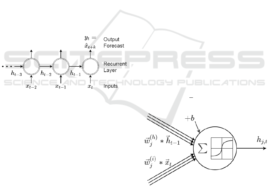
Figure 10: Unrolled representation of an RNN with one

recurrent layer. The x are vectors of inputs, the h the hidden

layer value vectors and y is the output, in our case a forecast

k time steps into the future.

The structure of a recurrent neural network is

sketched in Figure 10. For each time step the inputs

go to the recurrent layer, together with the outputs of

the recurrent layer in the previous time step. This is

done up to the last measurement, where the output

gives the forecast. The computation in the recurrent

layer is identical in each time-step, it consists of

several nodes, which can be visualized as in Figure

11. The components of the hidden layer vector 







are

calculated by equation 1:





 

















 



 













 







 





(1)

The 







and 



are adjustable weights and biases, 







is the input vector and 







is the output of the

recurrent layer of the last time step. 



is an

activation function, which has to be monotonically

rising. Typically, it is either a sigmoid function, or

even more simple, the ReLU function (Rectified

Linear Unit), defined by equation 2:











 









(2)

The weights of the inputs and of the hidden layer

outputs are shared between time steps. The output is

then calculated by a fully connected layer, mapping

the hidden layer values on the relevant output features

(equation 3):















 





 



(3)

With a large set of historical data, all weights and

biases are adjusted, to give the best fit on the known

outputs. This is done with an optimization algorithm

called backpropagation (Rumelhart et al., 1985).

The recurrent neural network can be extended in

different ways, for example by using multiple

recurrent layers, stacked one after the other. Another,

very popular extension is long short-term memory

(LSTM) networks. There, the node as shown in

Figure 11 is replaced by multiple computation steps.

Multiplication of the end values allows to only use

nodes when they are appropriate (Hochreiter and

Schmidhuber, 1997)(Sak et al., 2014).

The neural network has to be adjusted, to give the

best possible results. In our case, optimization is done

on the Mean Squared Error of the predicted value

(equation 4):

 













  











(4)

Figure 11: Visualization of the computation in a hidden

layer node. w denote weights, b bias, x inputs and h the

hidden layer values. j is the index of the node in the layer,

while t is the time index.

The performance of the RNN will be compared to

a naïve approach. For the naïve approach, forecasts

are produced that are equal to the last observed value.

SMARTGREENS 2018 - 7th International Conference on Smart Cities and Green ICT Systems

290

3.3 Use Case Definition

A first use case was defined to show the general

applicability of the proposed method. The simulated

scenario consists of a time series of partly cloudy

days. 10 measurement points are distributed in 5 km

distances on a line, with a non-changing cloud speed

of 9.3 m/s along this line. An equivalent scenario is

visualized in Figure 5. 10000 measurements of

minute averages are simulated. Results of forecasts of

one station for horizons from 1 to 15 minutes are

compared against a naïve forecast, and against results

of a neural network only using the local

measurements.

This scenario already includes the diurnal cycle of

PV production, as well as spatio-temporal

relationships and some mostly random differences

between the measurement stations. It can be seen as

the perfect scenario for the algorithm to be trained:

Partly cloudy conditions on a day with a steady wind

speed. Of course, there are a lot more influences in a

real scenario: Change in wind speed and direction,

two-dimensional and unregularly distributed PV

systems, differences in PV declination and

perturbations of the PV systems. Also cloud

formation and dissipation are not included, but should

not make a large difference on small time scales,

while on clear and overcast days the improvement of

the extended method will be minimal. Despite all of

this further challenges, the result on the single-

dimensional scenario shows already if recurrent

neural networks can be a promising approach for

forecasting from multiple PV measurement stations.

In a next step, the scenario is extended to two-

dimensions, where wind speed and direction changes

can be included. This simulation is done in Processing

(“Processing.org,” n.d.), using a Perlin Noise

implementation to simulate moving random cloud

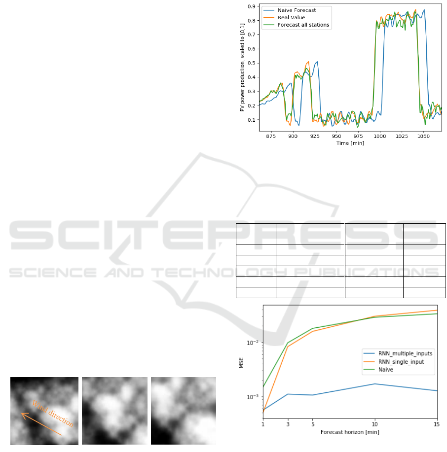
fields (Perlin, 1985) (see Figure 12).

Figure 12: Simulation of a moving cloud field with Perlin

Noise and Processing.

3.4 Preliminary Results

Figure 13 shows 10 minute forecasts for half a day of

partly cloudy weather. There it can be seen that the

RNN with multiple input stations successfully

forecasts abrupt PV generation changes. This is

facilitated by the measurements of stations, who are

reached earlier by the affecting cloud. In contrast the

naïve forecast (and similar other local forecast

methods) has a delay in the size of the forecasting

horizon.

Figure 13: Exemplary forecast for half a day, with a forecast

horizon of 10 mins. The RNN Forecast with all stations

manages to predict sudden changes quite precise.

Table 1: Mean squared error for three different models and

forecast horizons between 1 and 15 minutes.

RNN

Multiple inp

RNN

Single inp

Naïve

1 min

0.0558

0.0493

0.1473

3 min

0.1106

0.8299

0.9773

5 min

0.1064

1.5868

1.8033

10 min

0.1712

3.0243

2.8901

15 min

0.1277

3.8968

3.3475

Figure 14: Mean squared error of different forecast models,

plotted over the forecast horizon. MSE calculated excluding

night periods.

The Mean Squared Error (MSE) for multiple

forecasting horizons are shown in Table 1 and Figure

14. The RNN results are compared with the naïve

method, which takes the last measured value as

forecast, and an RNN with only the local PV inverter

Concept for Intra-Hour PV Generation Forecast based on Distributed PV Inverter Data

291

measurements and the hour of day as an input. The

simple RNN beats the naïve method only for really

short forecast horizons, as the temporal relationship

in our simulated data set is mostly random on longer

time scales. This is supposed to change for real data,

as there the network can learn time trends for different

weather regimes.

In comparison to those two methods, the RNN

with all 10 stations as input manages a big

improvement, especially for longer time horizons.

For horizons above 5 minutes the MSE is reduced to

less than 1/10. This is a significant improvement,

indicating that there also may be an improvement for

more difficult scenarios.

The final model uses the last 50 time steps and one

hidden layer with 40 neurons for prediction.

Furthermore, the hour of the day is included as an

input variable. LSTM models were tested in this

scenario and gave similar results as the RNN. For

more difficult scenarios it would be important to

include more training data, then also the differences

between LSTM and RNN could get more obvious.

4 DISCUSSION & OUTLOOK

A concept for an intra-hour forecast method using

distributed data from PV inverters and machine

learning techniques was introduced in this paper. The

concept assumes the option for PV systems to

broadcast their real-time power generation values and

the ability to receive such values from neighbouring

PV systems. As forecasting method, recurrent

neuronal networks were used. A simplified use-case

for a first proof of concept was created, by using

generic cloud movement at a constant wind speed and

direction.

The requirement analysis stresses the need for

data submissions from PV systems for at least every

minute for intra hour forecasts. The specific

minimum distances between neighboring systems are

depending on wind speed, data transmission rate and

a specific forecast horizon. For a 15 minutes forecast

horizon, distances would range from 5 up to 12 km

between systems, depending on the wind speed and

the corresponding movement of clouds.

A simplified use-case for a first proof of concept

was created, by using generic cloud movement at a

constant wind speed and direction. As forecasting

method, recurrent neuronal networks were used, as

they are designed to handle time series data. The

network can adapt to the time delayed relationship

between different PV stations and increases

forecasting accuracy by a factor of 10 in our

simplified scenario for forecasting horizons between

5 and 15 minutes (in comparison to the Naïve

forecast). Building on these promising results tests on

more realistic scenarios will follow in future. Also,

the kind and design of the neural network used for this

application shall be reviewed in more depth.

The next step in development will focus on

adapting the methods on a two-dimensional model of

25 PV systems arranged in a 5x5 grid. The movement

of clouds will again be simulated by using Processing

and Perlin Noise including changes of wind direction

and speed. Presumed that the neuronal networks

training on the data of this advanced use-case show

good results, a training set consisting of real measured

inverter data will be prepared for further

developments of the method.

ACKNOWLEDGEMENTS

This project has received funding in the framework of

the joint programming initiative ERA-Net Smart

Grids Plus, with support from the European Union’s

Horizon 2020 research and innovation programme.

REFERENCES

Antonanzas, J., Osorio, N., Escobar, R., Urraca, R.,

Martinez-de-Pison, F.J., Antonanzas-Torres, F., 2016.

Review of photovoltaic power forecasting. Sol. Energy

136, 78–111.

https://doi.org/10.1016/j.solener.2016.06.069.

Bessa, R.J., Trindade, A., Miranda, V., 2015. Spatial-

Temporal Solar Power Forecasting for Smart Grids.

IEEE Trans. Ind. Inform. 11, 232–241.

https://doi.org/10.1109/TII.2014.2365703.

E-Control Position Paper Tarife 2.0 [WWW Document],

n.d. E-Control Position Pap. Tarife 20. URL

https://www.e-

control.at/marktteilnehmer/strom/netzentgelte/tarife-2-

0 (accessed 11.29.17).

Graves, A., Mohamed, A. r, Hinton, G., 2013. Speech

recognition with deep recurrent neural networks, in:

2013 IEEE International Conference on Acoustics,

Speech and Signal Processing. Presented at the 2013

IEEE International Conference on Acoustics, Speech

and Signal Processing, pp. 6645–6649.

https://doi.org/10.1109/ICASSP.2013.6638947.

Hochreiter, S., Schmidhuber, J., 1997. Long Short-Term

Memory. Neural Comput. 9, 1735–1780.

https://doi.org/10.1162/neco.1997.9.8.1735.

SMARTGREENS 2018 - 7th International Conference on Smart Cities and Green ICT Systems

292

Lappalainen, K., Valkealahti, S., 2016. Apparent velocity

of shadow edges caused by moving clouds. Sol. Energy

138, 47–52.

https://doi.org/10.1016/j.solener.2016.09.008.

Lonij, V.P.A., Brooks, A.E., Cronin, A.D., Leuthold, M.,

Koch, K., 2013. Intra-hour forecasts of solar power

production using measurements from a network of

irradiance sensors. Sol. Energy 97, 58–66.

https://doi.org/10.1016/j.solener.2013.08.002.

Meteorological Network — ZAMG [WWW Document],

2017. URL

https://www.zamg.ac.at/cms/en/climate/meteorologica

l-network (accessed 11.20.17).

Perlin, K., 1985. An Image Synthesizer, in: Proceedings of

the 12th Annual Conference on Computer Graphics and

Interactive Techniques, SIGGRAPH ’85. ACM, New

York, NY, USA, pp. 287–296.

https://doi.org/10.1145/325334.325247.

Photovoltaik Karten [WWW Document], 2017. URL

https://www.klimafonds.gv.at/foerderungen/foerderlan

dkarte/photovoltaik-karten/ (accessed 11.20.17).

Processing.org [WWW Document], n.d. URL

https://processing.org/download/ (accessed 11.29.17).

Rumelhart, D.E., Hinton, G.E., Williams, R.J., 1985.

Learning Internal Representations by Error Propagation

(No. ICS-8506). California Univ. San Diego La Jolla

Inst. for Cognitive Science.

Sak, H., Senior, A., Beaufays, F., 2014. Long Short-Term

Memory Based Recurrent Neural Network

Architectures for Large Vocabulary Speech

Recognition. ArXiv14021128 Cs Stat.

TensorFlow [WWW Document], n.d. TensorFlow. URL

https://www.tensorflow.org/ (accessed 11.20.17).

Williamson, R.C., 2016. Machine-learning-based

forecasting of distributed solar energy production.

Windatlas Austria [WWW Document], n.d. Wind. Potential

Austria. URL

http://ispacevm11.researchstudio.at/index_v.html

(accessed 11.20.17).

APPENDIX

0,2

0,4

0,6

0,8

06:00 08:00 10:00 12:00 14:00 16:00 18:00

PV1

0,2

0,4

0,6

0,8

06:00 08:00 10:00 12:00 14:00 16:00 18:00

PV2

0,2

0,4

0,6

0,8

06:00 08:00 10:00 12:00 14:00 16:00 18:00

PV3

Concept for Intra-Hour PV Generation Forecast based on Distributed PV Inverter Data

293