Classification Analysis of NDVI Time Series in Metric Spaces for
Sugarcane Identification
Lucas Felipe Kunze, Th
´
abata Amaral, Leonardo Mauro Pereira Moraes,
Jadson Jos
´
e Monteiro Oliveira, Altamir Gomes Bispo Junior,
Elaine Parros Machado de Sousa and Robson Leonardo Ferreira Cordeiro
Institute of Mathematics and Computer Sciences, University of Sao Paulo,
Av. Trabalhador Sancarlense, 400, Sao Carlos, SP, Brazil
Keywords:
Data Mining, Classification, NDVI Time Series, Metric Space.
Abstract:
In Brazil, agribusiness is an important task for the economy, since it provides a substantial part of the coun-
try’s Gross Domestic Product. Besides that, interest in biofuels has grown, considering they make viable the
use of renewable energy. Brazil is the world’s largest producer of sugarcane, which enables a large ethanol
production. Thus, to monitor agricultural areas is important to support decision making. However, the amount
of generated and stored data about these areas has been increasing in such a way that far exceeds the human
capacity to manually analyze and extract information from it. That is why automatic and scalable data mining
approaches are necessary. This work focuses on the sugarcane classification task, taking as input NDVI time
series extracted from remote sensing images. Existing related works propose to analyze non-metric features
spaces using the DTW distance function as a basis. Here we demonstrate that analyzing the multidimensi-
onal space with Minkowski distance provides better results, considering a variety of classifiers. kNN using
L
2
distance performed similarly or better than using DTW. We also demonstrate a data configuration with
geolocation for training XGBoost, with results better than state-of-the-art.
1 INTRODUCTION
In recent years, the impacts caused by global warming
and climate changes have been highlighted. In this
sense, interest in biofuels has grown since they are
crucial to reduce greenhouse gases emissions by the
reason they make viable the use of renewable energy
instead of fossil fuels.
Brazil has some peculiarities (i.e. favorable cli-
mate, soil, water abundance, relief and luminosity)
that contribute to the development of agribusiness.
In 2016, the sector accounted for 23% of the coun-
try’s Gross Domestic Product (GDP), which is equi-
valent to USD 413.8 billion (Brasil, 2016; Bank,
2017). Brasil is the world’s leading producer of sugar-
cane (Service, 2017), which propitiates ethanol pro-
duction. In this way, considering the large Brazilian
territorial extension, it is relevant for the local govern-
ment and companies related to agriculture to monitor
those areas over the years, as to perform studies such
as production estimation, expansion identification, as
well as providing relevant information to support de-
cision making for agricultural producers and/or fun-
ding agencies.
However, the volume of data that is currently ex-
tracted from these areas, like satellite images, easily
reaches the hundreds of megabytes for storage and
millions of instances to process, which exceeds the
human capacity of manually analyze and extract sig-
nificant information from them. That is why levera-
ging data mining methods, such as clustering (Kyrgy-
zov et al., 2007) and classification (Julea et al., 2011)
is almost mandatory in this setting.
Considering the temporal information within
those data and applying data mining methods, sugar-
cane areas are commonly identified and monitored.
Usually it is used satellite images to monitor these
crops. This analysis aims to consider, for each sub-
area of the region of interest, corresponding to one
pixel of a satellite image, a series of values that indi-
cate the vegetation behavior of that subarea in a cer-
tain period of time. Information about vegetation is
usually obtained from the Normalized Difference Ve-
getation Index (NDVI) (Price, 1993). NDVI is rela-
ted to the amount and concentration of vegetation bi-
omass and it is widely used in agricultural researches
162
Kunze, L., Amaral, T., Mauro Pereira Moraes, L., José Monteiro Oliveira, J., Gomes Bispo Junior, A., Parros Machado de Sousa, E. and Cordeiro, R.
Classification Analysis of NDVI Time Series in Metric Spaces for Sugarcane Identification.
DOI: 10.5220/0006709401620169
In Proceedings of the 20th International Conference on Enterprise Information Systems (ICEIS 2018), pages 162-169
ISBN: 978-989-758-298-1
Copyright
c
 2019 by SCITEPRESS – Science and Technology Publications, Lda. All rights reserved

(da Silva et al., 2011; Scrivani et al., 2017; Jo
˜
ao et al.,
2018). In this sense, it is possible to differentiate su-
garcane areas from native forests, since they have dis-
tinct behaviors.
There are many researches that use NDVI as a
measure to classify or cluster crops (Romani et al.,
2011; da Silva et al., 2011; Amaral et al., 2014),
and most of them employ non-metric space analysis
and normally obtain their best results by using the
Dynamic Time Warping (DTW) to measure the dis-
tance between two time series. Sugarcane classifi-
cation methods that employ distances such as DTW
have some drawbacks, since its time complexity is
quadratic. Another reason is that DTW is not per-
formed on a metric space and, thus, cannot benefit
from improvements in speed on the same scale that
other methods performed on a metric space do. By its
definition, the metric space is a set with a metric dis-
tance that respects the following characteristics: non-
negativity, symmetry, triangular inequality and iden-
tity. Using these properties, pruning methods can be
applied (Mao et al., 2016).
These constraints make the investigation of via-
ble alternatives to DTW-based methods for sugarcane
classification in time series a task to be seriously con-
sidered. The same can be said for the choice of dis-
tance functions to be used by the classifier, conside-
ring the general speed advantages of metric spaces,
such as fast indexing of data and efficient pruning.
In this work, we perform the aforementioned in-
vestigation and aim to clarify those assumptions. Are
DTW-based methods, which take advantage of tem-
poral relations, unmatched in terms of accuracy, pre-
cision and recall or, if otherwise, what other methods
have comparable results? We begin from the hypothe-
sis that the DTW, considering the main features that
are desirable for a classifier, is not a prime choice for
sugarcane time series classification and that L
p
dis-
tances, when combined with adequate classifiers, are
viable options for this classification task.
This paper is organized as follows. Section 2
presents the Related Works and Section 3 describes
Background concepts that allows a better understan-
ding about the approach. Section 4 details how the in-
vestigation was conducted, including the dataset ana-
lysis, followed by Section 5 which explain the experi-
ments and results. After all, the Conclusions are pre-
sented in Section 6.
2 RELATED WORK
Satellites are important for agribusiness, since they
allow the remote sensing of regions (Romani et al.,
2011; da Silva et al., 2011; Amaral et al., 2014; Scri-
vani et al., 2017; do Valle Gonc¸alves et al., 2017).
Additionally, they make feasible free access to data.
In this way, agricultural producers can monitor their
crops, identify anomalies and take corrective actions
throughout the harvest, obtaining better productivity
results (Amaral et al., 2014).
Many researches in the literature idealize the cre-
ation of computational tools to semi-automatically
identify and monitor agricultural cultures, such as su-
garcane. The main difficulty of this task lies in the
small amount of labeled data compared to the total
amount of data (Amaral et al., 2014). An author
(Amaral et al., 2014) introduced a new framework to
classify sugarcane crops. In (da Silva et al., 2011), it
is proposed a supervised approach based on features
extraction to the coefficients obtained by time series
in Fourier decomposition.
In (Scrivani et al., 2017), the authors employ time
series for generating mathematical models that es-
timate sugarcane production using linear regression
with the following variables: NDVI / MODIS, Water
Requirement Satisfaction Index (WRSI), planted area
and sugarcane production. Their paper evidenced that
NDVI and WRSI are representative variables for ana-
lyzing sugarcane regions with one-year period time
series.
The work of (do Valle Gonc¸alves et al., 2017) des-
cribes a methodology that comprises two main pro-
cesses. The first one is the satellite images prepro-
cessing, where images are converted into SITS. The
second process employs clustering method on NDVI
time series, following the principle that time series are
grouped by their similarity. NDVI series are cluste-
red by the k-means algorithm under the DTW distance
function. The purpose is to analyze NDVI time series
of one or more sugarcane crop seasons.
Another approach for classifying NDVI time se-
ries uses association rules (Jo
˜
ao et al., 2018). The re-
searchers (Jo
˜
ao et al., 2018) analyzed their method’s
accuracy results using some traditional approaches,
such as Naive Bayes (NB), Random Forest (RF) and
Support Vector Machine (SVM). They demonstrated
that these traditional approaches do not attain an accu-
racy average higher than 55%.
3 BACKGROUND
3.1 Temporal Data
Temporal data are frequent in a variety of fields, such
as economics (e.g. number of sales, price of pro-
ducts), medicine (e.g. disease detection, patient pro-
Classification Analysis of NDVI Time Series in Metric Spaces for Sugarcane Identification
163

gress evaluation) and agrometeorology (e.g. evolution
of a given crop) (Maimon and Rokach, 2005; Mitsa,
2010).
According to (Mitsa, 2010; Esling and Agon,
2012), time series is the most common type of tem-
poral data and they represent ordered real-valued me-
asurements at regular or irregular temporal intervals.
A time series can be univariate or multivariate. If only
one variable is used to construct time series, it is cal-
led univariate, otherwise, we have a multivariate time
series.
A univariate time series T s is defined as T s =
[(t
1
,v
1
),(t
2
,v
2
),...,(t
n
,v
n
)] and, for each time t
i
,
where i assumes a value in the range 1 ≤ i ≤ n, there
is a value v
i
associated.
3.2 Classification
Classification consists in the task of assigning a new
sample to a set of previously known classes (Mitsa,
2010). Because of the supervised nature of this task,
additional knowledge about the problem must be ta-
ken into account. This knowledge can be obtained by
domain experts or by a sample of labeled data, which
is commonly referred as the training dataset.
The classification algorithms used in this work
are: k-Nearest Neighbors (kNN) (Cover and Hart,
1967), Naive Bayes (NB) (Larsen, 2005), Decision
Trees (DT) (Tanha et al., 2017), Multilayer Percep-
tron (MLP) (Boughrara et al., 2017) and Extreme
Gradient Boosting (XGBoost) (Chen and He, 2015).
The kNN technique consists in an algorithm that
makes predictions based on the instances stored in
the dataset. The NB classifier consists in a statisti-
cal approach (Larsen, 2005). Decision Trees is an ap-
proach that aims to divide a complex decision into a
set of simpler decisions (Tanha et al., 2017; Mitsa,
2010). MLP consists in a neural network which are
suited to solve problems that are not linearly separa-
ble (Boughrara et al., 2017). XGBoost, a scalable and
portable approach based on Gradient Boosting, con-
sists in an ensemble of other prediction models (e.g.
CART Trees) (Chen and He, 2015).
3.3 Distance Functions
Distance functions measure how much the objects are
distant. In classification task, they are useful to check
how distant (or dissimilar) two objects are, and choo-
sing the correct function is essential to obtain high-
quality results. Advantages and limitations of each
function should be considered, as well as the nature
of the data to be analyzed.
There is a wide variety of distance functions, for
example the Minkowski distance (L
p
) that is a metric
in a normed vector space. Given two vectors of real
numbers A = {a
1
,a
2
,..., a
n
} and B = {b
1
,b
2
,. .., b
n
},
the Minkowski distance is formalized by:
L
p
=
n
∑
i=1
|a
i
− b
i
|
p
!
1/p
(1)
However, the Minkowski distances concentrate at
calculating the direct distance between two vector
points, wherein the vectors must have the same ba-
seline, scale and length (Mitsa, 2010). An alterna-
tive is Dynamic Time Warping (DTW), which con-
sists in a non-linear distance function that uses dyna-
mic programming to find the best alignment between
time series, not necessarily with the same length each
other. Given two time series X = {x
1
,x
2
,. .., x
r
} and
Y = {y
1
,y
2
,. .., y
s
}, the DTW (X,Y ) cost of a warping
path P between X and Y is defined by:
DTW (X ,Y ) = min
P
∑
p=1
γ(x
i
p
,y
j
p
) (2)
This warping path aims to evaluate the recurrence,
using dynamic programming (Ratanamahatana and
Keogh, 2004). Where γ(x
i
,y
j
) is the cumulative dis-
tance of d(x
i
,y
j
) and the minimum cumulative dis-
tances from up to three forwardly adjacent cells (Kim
et al., 2001).
3.4 Satellite Image Time Series
This work used satellites with low spatial resolution
and high temporal resolution images, namely the Ad-
vanced Very High Resolution Radiometer (AVHRR)
sensor, aboard the National Oceanic and Atmospheric
Administration (NOAA) satellite.
A common approach in satellite image analysis
consists in classifying each pixel or a subset of pixels
from an image using data mining techniques (Romani
et al., 2011; da Silva et al., 2011; Scrivani et al., 2017;
do Valle Gonc¸alves et al., 2017; Jo
˜
ao et al., 2018). In
the context of this work, we used a method oriented to
Satellite Image Time Series (SITS), where time series
are generated by one-year period, corresponding to a
twelve monthly satellite images from April to March
of 2004/2005.
For these images, each pixel represents a region
of approximately 1km x 1km and has a NDVI value
associated with its respective real coordinate. In this
way, each pixel is represented by a time series T s =
[(t
1
,v
1
),(t
2
,v
2
),. .., (t
12
,v
12
)]. We conduct this work
with the same dataset used in (Amaral et al., 2014)
ICEIS 2018 - 20th International Conference on Enterprise Information Systems
164

which contains images and geographical informations
about Sao Paulo/Brazil provided by Embrapa
1
.
4 PROPOSED INVESTIGATION
4.1 Dataset Analysis
This analysis aims to examine the classes in dataset.
Table 1 shows the classes distribution, and it is no-
table that the quantity of non-sugarcane instances is
greater than that of sugarcane instances. As such,
we observe the correlation between the sugarcane and
non-sugarcane classes. The instances used in this cor-
relation analysis were chosen manually by domain ex-
perts and it propitiates the creation of an ideal confi-
guration for applying the classification approach, con-
sidering the fact that the most representative instances
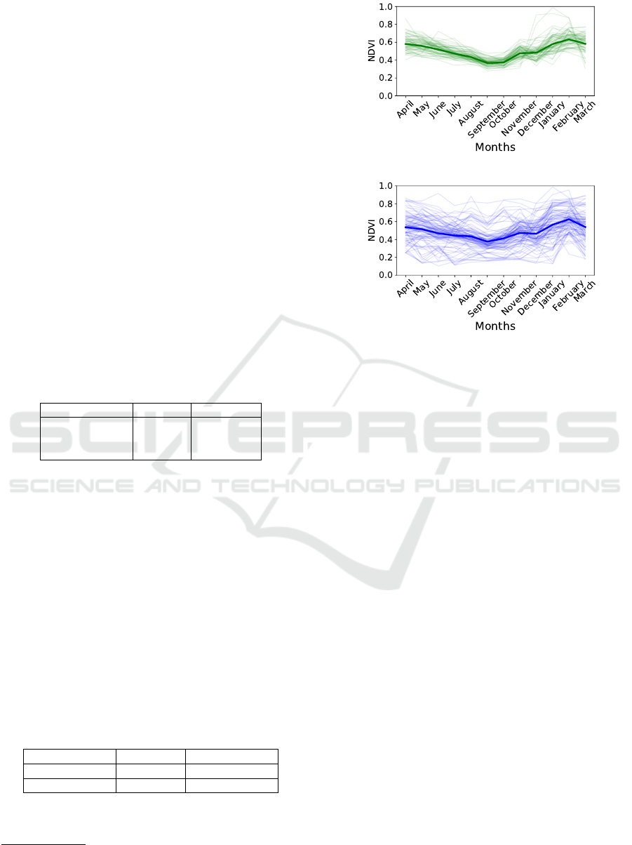
were selected. Figure 1.1 represents sugarcane time
series and Figure 1.2 corresponds to non-sugarcane
time series. Additionally, the NDVI average is indi-
cated by the highlighted line.
Table 1: Dataset: class proportion distribution.
Class Amount Proportion
Sugarcane 26.964 13.58%
Non-sugarcane 171.534 86.42%
Total 198.498 100.00%
Analyzing the graphs of Figure 1, it is possible to
infer that the NDVI average for the time series are ap-
proximately the same. To notice that, we calculated
the Pearson correlation between both classes. After
calculating the correlation between sugarcane instan-
ces, a bi-dimensional matrix was generated and the
average value from the lower triangle was extracted,
disregarding the main diagonal. The same process is
accomplished both for non-sugarcane instances and
sugarcane against non-sugarcane instances. The re-
sults are showed in Table 2 and they demonstrate that
elements in non-sugarcane class have lower correla-
tion values than non-sugarcane class if compared with
non-sugarcane/sugarcane.
Table 2: Pearson correlation between sugarcane and non-
sugarcane instances.
Class Sugarcane Non-sugarcane
Sugarcane 0.7399 0.6120
Non-sugarcane 0.6120 0.5312
1
Brazilian Agricultural Research Corporation.
https://www.embrapa.br/
(a) Sugarcane
(b) Non-sugarcane
Figure 1: Sugarcane Times Series x Non-Sugarcane Time
Series.
4.2 Geographical Coordinates
Assuming that sugarcane is grown throughout vast
and nearby areas, latitude and longitude of instan-
ces were added to the features vector in order to im-
prove the information gain. When DTW is computed,
its distance is incremented with L
2
calculations using
lat and lon values of the instance in question, where
[lat
x
,lon
x
] augments X and [lat
y
,lon
y
] augments Y .
DTW
locality
distance is defined by Equation 3:
DTW
locality
(X,Y ) = DTW (X ,Y )
+ L
2
([lat
x
,lon
x
] , [lat
y
,lon
y
])
(3)
L
p−locality
is an improvement by the actual lat
and lon values for each instance, such that it results
in the vectors X
locality
= [v
x1
,v
x2
,. .., v
x12
,lat
x
,lon
x
]
and Y
locality
= [v
y1
,v
y2
,. .., v
y12
,lat
y
,lon
y
]. At last, the
vectors with (lat and lon) augmentation are used in
L
p
(X
locality
,Y
locality
) distance function.
4.3 Evaluation Metrics
In order to evaluate the classification performance,
we calculated the Matthews Correlation Coefficient
(MCC) coefficient (Matthews, 1975), accuracy, recall
and precision (Maimon and Rokach, 2005).
Classification Analysis of NDVI Time Series in Metric Spaces for Sugarcane Identification
165

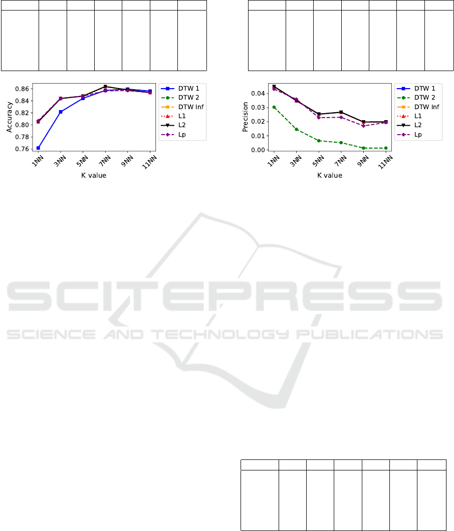
Table 3: Experiment 1: Accuracy.
Distance 1NN 3NN 5NN 7NN 9NN 11NN
DTW 1 0.761 0.821 0.844 0.857 0.859 0.856
DTW 2 0.805 0.843 0.846 0.863 0.858 0.853
DTW Inf 0.805 0.843 0.847 0.863 0.858 0.853
L
1
0.805 0.843 0.847 0.863 0.858 0.853
L
2
0.805 0.843 0.847 0.863 0.858 0.853
L
3
0.807 0.844 0.847 0.856 0.856 0.853
Table 4: Experiment 1: Precision.
Distance 1NN 3NN 5NN 7NN 9NN 11NN
DTW 1 0.045 0.034 0.025 0.026 0.019 0.019
DTW 2 0.030 0.014 0.006 0.005 0.001 0.001
DTW Inf 0.045 0.034 0.025 0.026 0.019 0.019
L
1
0.045 0.034 0.025 0.026 0.019 0.019
L
2
0.045 0.034 0.025 0.026 0.019 0.019
L
3
0.043 0.036 0.022 0.023 0.017 0.019
Figure 2: Experiment 1: Accuracy.
5 EXPERIMENTS AND RESULTS
We have conducted a set of experiments in order to
answer some questions about classification task in
NDVI time series for sugarcane identification. Those
experiments are described as follows:
• Experiment 1 was performed to evaluate the effi-
ciency of metric space distance functions, testing
variations of L
p
family and the DTW distance.
• Experiment 2 attempts to analyze if geographi-
cal location information can improve the perfor-
mance of the classification task.
• Experiment 3 aims to identify a good configura-
tion for the classifier training, considering sugar-
cane and non-sugarcane instances. Besides that,
it investigates the efficiency of some classification
algorithms and the impact that geographical lo-
cation information has on these classifiers. Also,
maximizing the MCC value by using predefined
parameters found in previous experiments. The
results of experiment are compared with state-of-
the-art.
In the experiments, the settings adopted by Multi-
layer Perceptron algorithm assumed one hidden layer
with 100 neurons, learning rate of 0.001 per iteration
and 100,000 as the max number of iterations. In case
of XGBoost, the used parameters are: 3 as max depth,
200 as estimator number and learning rate of 0,015.
kNN under some variations of k. Decision Tree uses
entropy. Finally, Naive Bayes’ standard configuration
doesn’t need parameters.
Figure 3: Experiment 1: Precision.
5.1 Experiment 1
In the first experiment, we evaluate some variations
of P to DTW and some variations of p to L
p
distan-
ces. The propose of this experiments are the compute
efficiency of DTW and L
p
. The tests were conducted
under DTW distance, which is traditionally used to
compare time series. The objective is to evaluate its
performance compared with the distance algorithms
for multidimensional spaces (i.e. Minkowski family
distances). To perform this experiment, we used 200
random instances for training and 10,000 random in-
stances for testing. This procedure was performed 10
times and the final results are the average of the itera-
tion results. The k NN = {1, 3,5,7, 9,11} was perfor-
med under the DTW and L
p
distances, where DTW
used the following configurations: P = 1 (DTW 1),
P = 2 (DTW 2) and P = ∞ (DTW Inf), while the L
p
was performed with p = 1 (Manhattan distance / L
1
),
p = 2 (Euclidean distance / L
2
) and p = 3 (L
3
).
Table 5: Experiment 1: Recall.
Distance 1NN 3NN 5NN 7NN 9NN 11NN
DTW 1 0.270 0.217 0.161 0.176 0.126 0.122
DTW 2 0.170 0.086 0.041 0.033 0.008 0.007
DTW Inf 0.270 0.217 0.161 0.175 0.126 0.122
L
1
0.270 0.217 0.161 0.176 0.126 0.122
L
2
0.270 0.217 0.161 0.176 0.126 0.122
L
3
0.260 0.223 0.146 0.150 0.108 0.118
Table 3 and Figure 2 describe the general accuracy
of each algorithm using the aforementioned definiti-
ons. The first relevant observation is that DTW 2 and
DTW Inf presented high accuracy compared with the
DTW 1. In addition, it is visible that the algorithms
using L
p
distances in the multidimensional space pre-
sented similar accuracy matching the DTW approa-
ICEIS 2018 - 20th International Conference on Enterprise Information Systems
166

ches in all cases. In this way, we conclude that DTW
2 is sufficient for this context and L
p
distances have
results similar to those obtained using the DTW.
Table 4 and Figure 3 indicate the precision of the
evaluated algorithms. Relating Figure 3 to Figure 2, it
is possible to note that as the general accuracy incre-
ases, precision decreases and recall increases (Table
5). This condition directly affects the accuracy, since
the number of non-sugarcane instances is greater than
the number of sugarcane instances, as showed in the
Table 1.
In addition, observing the precision (Table 4) and
recall (Table 5), we noticed that the distances that pre-
sented the highest precision were the ones of the Min-
kowski family, standing out the L
2
distance that in al-
most all the kNN tests, presented the highest accu-
racy. Therefore, DTW does not present gain in this
application, since the multidimensional space distan-
ces presented better results without using the temporal
information itself.
5.2 Experiment 2
Another observation from Experiment 1 (Section 5.1),
kNN = 7 presented better results in terms of accuracy,
precision and recall. Therefore, the other experiments
adopted this configuration for kNN algorithm.
In Experiment 2 we will test the inclusion of lo-
cality in distance algorithms, as reported in Section
4.2. Appending the real geographical coordinate (i.e.
latitude and longitude) of the instances, a better in-
stances classification is expected, since sugarcane is
grown throughout nearby areas.
Analogously to the previous experiment, we tes-
ted DTW 1, DTW 2, DTW Inf, L
1
, L
2
and L
3
distance
functions. It also followed the setup of 200 random
instances for training and 10,000 random instances
for testing.
Table 6 presents the results obtained in this expe-
riment. Observing the accuracy in Table 6 and Table
3, we notice that in some algorithms there was an in-
crease in their accuracy. In addition, it is noted that
the precision and recall of the experiments with lo-
cality (Table 6) increased compared to the precision
(Table 4) of the experiments without locality. In this
way, the distance functions presented a better perfor-
mance with the addition of the locality, representing
an information gain.
Again, we can see that the distance L
2
stood out
in relation to the other distances, while the other ones
presented similar results. Thus, besides the fact that
distances of the multidimensional space have a lower
computational cost than DTW, they also presented su-
perior results, demonstrating that for the problem in
Table 6: Experiment 2: 7NN with distance using locality,
evaluating accuracy (Acc), precision, recall and MCC.
Distance Acc Precision Recall MCC
DTW 1 0.856 0.0344 0.2134 0.2449
DTW 2 0.860 0.0375 0.2457 0.2559
DTW Inf 0.862 0.0362 0.2333 0.2635
L
1
0.862 0.0359 0.2314 0.2636
L
2
0.864 0.0375 0.2426 0.2750
L
3
0.862 0.0366 0.2360 0.2635
question there was no advantage in using temporal in-
formation of the time series.
5.3 Experiment 3
In the previous experiment we concluded that use of
geographic coordinates gives better results. In the
current experiment, the objective is find the best ra-
tio for training between both classes, testing in some
classifiers (i.e. kNN, MLP, XGBoost, DT and NB).
To perform this experiment, we used 700 elements
to training, the ratio between positive and negative
r = {0.3, 0.4,0.5,0.6, 0.7}, and if the test data wit-
hout geographic information (Table 7 and Figure 4)
and with location (Table 8 and Figure 5). For this ex-
periment we used 1,000 elements for testing, and we
run all algorithms 10 times, and the average is extrac-
ted.
As verified in Experiment 2 (Section 5.2), using
location information is better than to do not use, and
the current experiment confirms that fact, since all
algorithms performed better with geographic infor-
mation, except MLP. Checking the average of higher
MCC values, it is possible to conclude that the best
positive ratio lies somewhere between 0.4 and 0.5.
Considering the two classifiers that obtained higher
MCC value (XGBoost and kNN L
2
), the best configu-
ration, using simple vote, has ratio 0.4. The current
experiment found the best distribution between clas-
ses, that is 40% of training set composed by class su-
garcane and 60% of class non-sugarcane and the Ex-
periment 4 assumes that ratio for the next tests.
After finding the best ratio value between both
classes, we want to know the effects of varying trai-
ning dataset sizes by several experiments analyzing
the performance of MCC. Observing Figure 6 it is
visible that as bigger the training dataset gets, better
the performance. However it is stabilized about sizes
1,000 to 3,000. It is interesting to observe that with
700 elements for training is possible to beat traditi-
onal algorithms that use non-metric distances which
MCC = 0.343 (Amaral et al., 2014). The kNN L
2
and
XGBoost beat with 0.363 and 0.360 respectively, and
other algorithms show good results but do not have
beat the state-of-the-art. Also, MLP lost in all cases.
Classification Analysis of NDVI Time Series in Metric Spaces for Sugarcane Identification
167

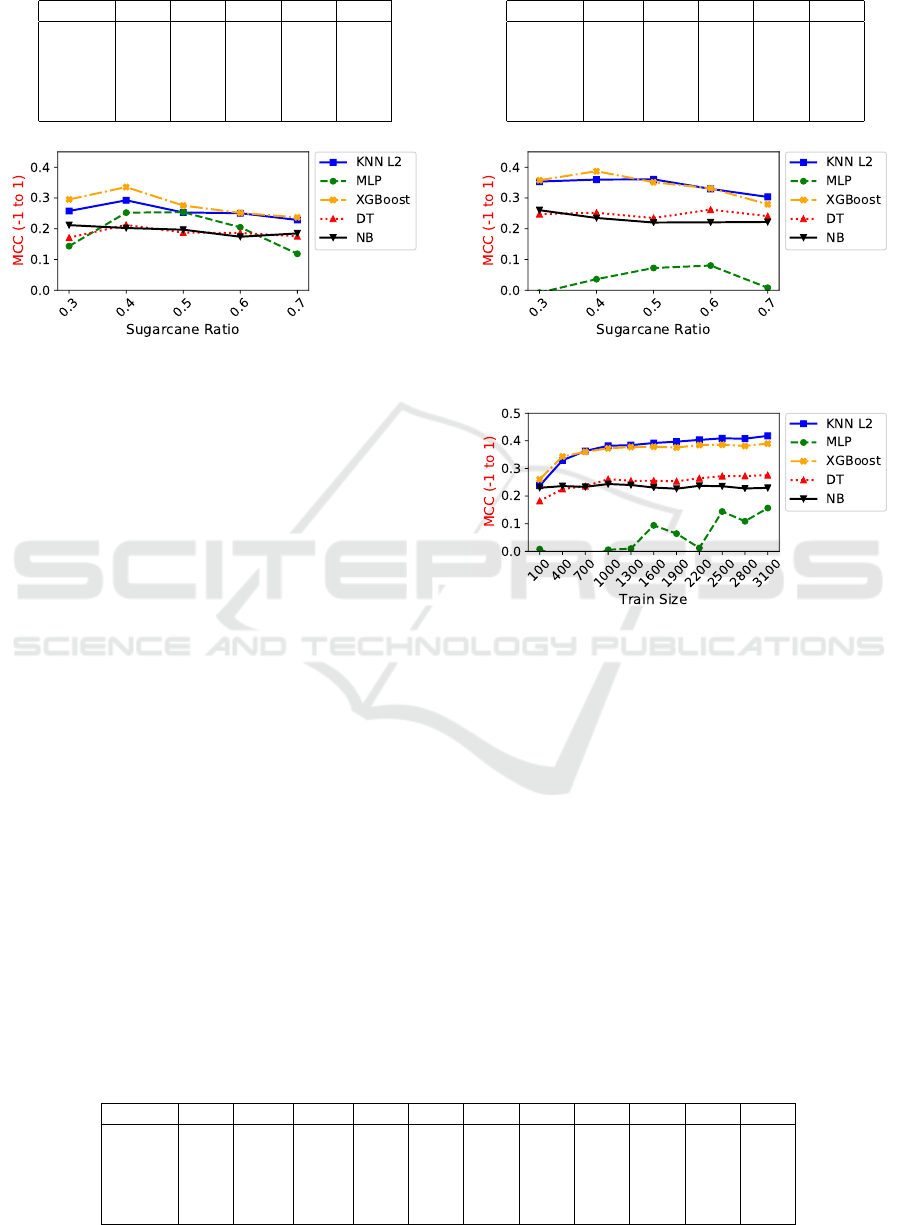
Table 7: Experiment 3: Evaluating MCC. Normal NDVI
time series.
Classifier 0.3 0.4 0.5 0.6 0.7
kNN L
2
0.257 0.292 0.252 0.25 0.228
MLP 0.143 0.252 0.253 0.204 0.118
XGBoost 0.295 0.335 0.275 0.251 0.236
DT 0.17 0.212 0.187 0.186 0.175
NB 0.211 0.202 0.196 0.173 0.184
Table 8: Experiment 3: Evaluating MCC. NDVI time series
with locality.
Classifier 0.3 0.4 0.5 0.6 0.7
kNN L
2
0.353 0.359 0.360 0.329 0.303
MLP -0.008 0.035 0.072 0.080 0.007
XGBoost 0.357 0.387 0.351 0.331 0.279
DT 0.247 0.251 0.234 0.262 0.240
NB 0.260 0.234 0.220 0.220 0.221
Figure 4: Experiment 3: Evaluating MCC. Normal NDVI
time series.
Figure 5: Experiment 3: Evaluating MCC. NDVI time se-
ries with locality.
6 CONCLUSIONS
Sugarcane classification is a very time-consuming
process when done manually. Thus, it is important
to develop scalable and efficient methods to accom-
plish this work. As the need for knowledge in agribu-
siness grows, crop classification remains an important
tool for the experts, since it allows the monitoring of
a culture that has high relevance in the economy of
Brazil.
We performed a series of experiments with several
combinations of classifiers (i.e. Naive Bayes, Deci-
sion Tree, Multilayer Perceptron, XGBoost an kNN)
and distance functions (i.e. L
1
, L
2
, L
p
and DTW),
and also the addition or not of geographic coordina-
tes into the input data that is sent to the classifier. We
have concluded that the use of geographic informa-
tion may help the sugarcane classification task and,
in fact, it did exactly that for the highest performing
classifiers in our experiments, namely XGBoost and
kNN using L
2
distance. The experimental results sho-
wed kNN using L
2
distance obtaining similar accu-
racy than kNN using DTW. kNN using DTW did not
outperform XGBoost or kNN L
2
in terms of accuracy,
precision, recall and MCC. Taking into account the
higher computational cost of DTW distance, we also
Figure 6: Experiment 3: Evaluating MCC. NDVI time se-
ries with locality, variating in training dataset size.
conclude that XGBoost and kNN using L
2
are better
choices than kNN using DTW. Also, XGBoost have
accuracy higher than state-of-the-art (Amaral et al.,
2014), for the task of sugarcane classification.
Since L
2
distance calculations are performed on a
metric space, they can benefit from the triangle ine-
quality property of metric spaces which allows pru-
ning of instances, thus speeding up the computations.
This is especially important for processing large data
volumes. This feature could be further explored by
a future work. We aim to apply indexing methods in
order to reduce the computational cost during classifi-
cation. Even at the point up to where we reached with
our experiments, the improvements in computational
cost for simply using a L
p
distance instead of DTW
are significant.
Table 9: Experiment 3: Evaluating MCC. NDVI time series with locality, variating in training dataset size.
Classifier 100 400 700 1000 1300 1600 1900 2200 2500 2800 3100
kNN L
2
0.237 0.329 0.363 0.382 0.384 0.392 0.396 0.403 0.408 0.407 0.417
MLP 0.007 -0.028 -0.026 0.005 0.009 0.094 0.064 0.012 0.144 0.108 0.156
XGBoost 0.260 0.342 0.360 0.372 0.377 0.378 0.375 0.384 0.385 0.381 0.389
DT 0.182 0.225 0.235 0.261 0.255 0.255 0.253 0.264 0.272 0.272 0.275
NB 0.229 0.236 0.233 0.243 0.240 0.23 0.226 0.237 0.235 0.227 0.229
ICEIS 2018 - 20th International Conference on Enterprise Information Systems
168

ACKNOWLEDGEMENTS
We thank National Council for Scientific and Techno-
logical Development (CNPq), National Council for
the Improvement of Higher Education (CAPES) and
Sao Paulo Research Foundation (FAPESP) for finan-
cial support.
REFERENCES
Amaral, B. F. d., Gonc¸alves, R., Romani, L., Sousa, E. P.
M. d., et al. (2014). Improving the semi-supervised
classification of time series extracted from satellite
images (in portuguese: Aprimorando a classificac¸
˜
ao
semissupervisionada de s
´
eries temporais extra
´
ıdas de
imagens de sat
´
elite). In Symposium on Knowledge
Discovery, Mining and Learning, 2th. Sociedade Bra-
sileira de Computac¸
˜
ao-SBC, KDD.
Bank, W. (2017). Databank - brazil. The World Bank
(IBRD - IDA) - https://data.worldbank.org/country/
brazil?locale=pt. Accessed: 2017-09-15.
Boughrara, H., Chtourou, M., and Amar, C. B. (2017). MLP
neural network using constructive training algorithm:
application to face recognition and facial expression
recognition. IJISTA, 16(1):53–79.
Brasil, G. (2016). Agribusiness may increase of 2% in 2017
(in portuguese: Agroneg
´
ocio deve ter crescimento de
2% em 2017). http://www.wpcentral.com/ie9-
windows-phone-7-adobe-flash-demos-and-
development-videos. Accessed: 2017-09-13.
Chen, T. and He, T. (2015). Xgboost: extreme gradient
boosting. R package version 0.4-2.
Cover, T. and Hart, P. (1967). Nearest neighbor pattern clas-
sification. IEEE transactions on information theory,
13(1):21–27.
da Silva, W. L., Gonc¸alves, R. R. V., Siqueira, A. S., Zullo,
J., and Neto, F. A. M. G. (2011). Feature extraction
for ndvi avhrr/noaa time series classification. In 2011
6th International Workshop on the Analysis of Multi-
temporal Remote Sensing Images (Multi-Temp), pages
233–236.
do Valle Gonc¸alves, R. R., Zullo, J., Romani, L. A. S.,
do Amaral, B. F., and Sousa, E. P. M. (2017). Agri-
cultural monitoring using clustering techniques on sa-
tellite image time series of low spatial resolution. In
2017 9th International Workshop on the Analysis of
Multitemporal Remote Sensing Images (MultiTemp),
pages 1–4, Brugge, Belgium.
Esling, P. and Agon, C. (2012). Time-series data mining.
ACM Computing Surveys (CSUR).
Jo
˜
ao, R. S., Mpinda, S. T. A., Vieira, A. P. B., Jo
˜
ao, R. S.,
Romani, L. A. S., and Ribeiro, M. X. (2018). A New
Approach to Classify Sugarcane Fields Based on As-
sociation Rules, pages 475–483. Springer Internatio-
nal Publishing, Cham.
Julea, A., Meger, N., Bolon, P., Rigotti, C., Doin, M. P.,
Lasserre, C., Trouve, E., and Lazarescu, V. N.
(2011). Unsupervised spatiotemporal mining of satel-
lite image time series using grouped frequent sequen-
tial patterns. IEEE Transactions on Geoscience and
Remote Sensing, 49(4):1417–1430.
Kim, S., Park, S., and Chu, W. W. (2001). An index-
based approach for similarity search supporting time
warping in large sequence databases. In Data Engi-
neering, 2001. Proceedings. 17th International Confe-
rence on, pages 607–614, Heidelberg, Germany, Ger-
many. International Conference on Data Engineering
(IEEE).
Kyrgyzov, I. O., Maitre, H., and Campedel, M. (2007). A
method of clustering combination applied to satellite
image analysis. In 14th International Conference on
Image Analysis and Processing (ICIAP 2007), pages
81–86.
Larsen, K. (2005). Generalized naive bayes classifiers.
SIGKDD Explorations, 7(1):76–81.
Maimon, O. and Rokach, L. (2005). The Data Mining and
Knowledge Discovery Handbook. Springer.
Mao, R., Zhang, P., Li, X., Liu, X., and Lu, M. (2016).
Pivot selection for metric-space indexing. Internati-
onal Journal of Machine Learning and Cybernetics,
7(2):311–323.
Matthews, B. W. (1975). Comparison of the predicted and
observed secondary structure of t4 phage lysozyme.
Biochimica et Biophysica Acta (BBA)-Protein Struc-
ture, 405(2):442–451.
Mitsa, T. (2010). Temporal data mining. CRC Press.
Price, J. C. (1993). Estimating leaf area index from satellite
data. IEEE Transactions on Geoscience and Remote
Sensing, 31(3):727–734.
Ratanamahatana, C. A. and Keogh, E. (2004). Everything
you know about dynamic time warping is wrong. In
Third Workshop on Mining Temporal and Sequential
Data, pages 22–25. Citeseer.
Romani, L. A. S., Gonc¸alves, R. R. V., Amaral, B. F., Chino,
D. Y. T., Zullo, J., Traina, C., Sousa, E. P. M., and
Traina, A. J. M. (2011). Clustering analysis applied to
ndvi/noaa multitemporal images to improve the moni-
toring process of sugarcane crops. In 2011 6th Inter-
national Workshop on the Analysis of Multi-temporal
Remote Sensing Images (Multi-Temp), pages 33–36.
Scrivani, R., Zullo, J., and Romani, L. A. S. (2017). Sits
for estimating sugarcane production. In 2017 9th In-
ternational Workshop on the Analysis of Multitempo-
ral Remote Sensing Images (MultiTemp), pages 1–4,
Brugge, Belgium.
Service, F. A. (2017). Sugar: World markets and
trade. United States Department of Agriculture -
https://apps.fas.usda.gov/psdonline/circulars/sugar.pdf.
Accessed: 2017-10-10.
Tanha, J., van Someren, M., and Afsarmanesh, H. (2017).
Semi-supervised self-training for decision tree clas-
sifiers. Int. J. Machine Learning & Cybernetics,
8(1):355–370.
Classification Analysis of NDVI Time Series in Metric Spaces for Sugarcane Identification
169