Non-intrusive Distracted Driving Detection based on

Driving Sensing Data

Sasan Jafarnejad, German Castignani and Thomas Engel

Interdiscipl. Centre for Security, Reliability & Trust (SnT), University of Luxembourg, Esch-Sur-Alzette, Luxembourg

Keywords:

Distraction, Inattention, Driver Behavior, Machine Learning, Driver Modeling.

Abstract:

Nowadays Internet-enabled phones have become ubiquitous, and we all witness the ﬂood of information that

often arrives with a notiﬁcation. Most of us immediately divert our attention to our phones even when we

are behind the wheel. Statistics show that drivers use their phone on 88% of their trips, in 2015 in the United

Kingdom 25% of the fatal accidents were caused by distraction or impairment. Therefore there is need to tackle

this issue. However, most of the distraction detection methods either use expensive dedicated hardware and/or

they make use of intrusive or uncomfortable sensors. We propose a distracted driving detection mechanism

using non-intrusive vehicle sensor data. In the proposed method 8 driving signals are used. The data is

collected, then two sets of statistical and cepstral features are extracted using a sliding window process, further

a classiﬁer makes a prediction for each window frame, lastly, a decision function takes the last l predictions

and makes the ﬁnal prediction. We evaluate the subject independent performance of the proposed mechanism

using a driving dataset consisting of 13 drivers. We show that performance increases as the decision window

gets larger. We achieve the best results using a Gradient Boosting classiﬁer with a decision window of total

duration 285 seconds which yields ROC AUC of 98.7%.

1 INTRODUCTION

Nowadays Internet-enabled smart-phones have be-

come ubiquitous, and we all witness the ﬂood of in-

formation that often arrives with a notiﬁcation. Most

of us immediately divert our attention to our smart-

phones regardless of what we are doing and fre-

quently we do so even when we are behind the wheel.

A recent study have shown that drivers use their

phones in about 88% of their trips, and in average

they spend in 3.5 minutes of each hour of driving on

their phone

. Although mobile-phone related distrac-

tions are only a subset of all driving distractions, it

has been proven that driving distractions are danger-

ous to passenger safety (Klauer et al., 2010). Recent

statistics indicate that a large portion of fatal accidents

are caused due to driver distractions. For example

according to Department of Transport of the United

Kingdom, in 2015 about 25% of fatal accidents were

caused by distraction or impairment

. This implies

that any solution that mitigates distracted driving even

by a small amount can save lives. This motivates us to

http://blog.zendrive.com/distracted-driving/

https://www.gov.uk/government/statistics/reported-

road-casualties-great-britain-annual-report-2015

propose a distracted driving detection mechanism that

is able to detect and warn the driver at such moments

and can be available for the majority of car owners.

Although this work is not the ﬁrst attempt at solv-

ing this problem, it follows a novel and ambitious ap-

proach. Current literature mostly uses dedicated sen-

sors to detect distractions, sensors such as cameras

for tracking head orientation (W

ollmer et al., 2011) or

measuring the skin temperature (Wesley et al., 2010),

however we propose to only use the standard vehicle

sensors, therefore this method could be applicable to

the most of the commercial vehicles on the market.

In this approach we do not use any intrusive sen-

sors such as cameras or microphones, instead we fo-

cus on car driving data. We aim to classify driving

segments as distracted or not distracted driving. Such

a system can be used on-line to alert the driver in

case of continuous distraction. Or alternatively can

be employed off-line as a metric to judge the driv-

ing performance or for risk assessment of the driver.

First we use a sliding window to extract features from

driving signals, then using machine learning we clas-

sify each window as distracted or not-distracted, then

we use a decision function to decide whether a se-

quence of window frames represent distracted driving

178

Jafarnejad, S., Castignani, G. and Engel, T.

Non-intrusive Distracted Driving Detection based on Driving Sensing Data.

DOI: 10.5220/0006708401780186

In Proceedings of the 4th International Conference on Vehicle Technology and Intelligent Transport Systems (VEHITS 2018), pages 178-186

ISBN: 978-989-758-293-6

or not. We propose to validate this method using driv-

ing traces from 13 drivers chosen from a large driving

dataset called UYANIK (Abut et al., 2007). For eval-

uation we present the performance of the proposed

method in terms of F

score and area under the Re-

ceiver Operating Characteristic curve (ROC AUC).

The remainder of the paper is organized as fol-

lows, at Section 2 we present an overview of the prior

work on distraction detection that is relevant to this

work, in Section 3 we describe the dataset used for

validation, next in Section 4 we describe our proposed

methodology and the evaluation strategy. In Section 5

we present the evaluation results and in Section 6 we

discuss the obtained results. Lastly in Section 7 we

conclude and present the future directions.

2 RELATED WORK

Researchers have been trying to reach a consensus for

the deﬁnition of distracted driving however although

there have been many attempts at formalizing dis-

tracted driving there are still discussions around this

subject. Inattention is a major cause of unsafe driv-

ing and accidents, however inattention itself can be

caused by various means. According to the latest

driver inattention taxonomy from the United States

and European Union Bilateral Intelligent Transporta-

tion Systems Task Force (Engstr

om et al., 2013)

driver drowsiness and driver distraction are two ma-

jor processes that give rise to inattention. There is a

large body of research in the literature attending to

both drowsiness and distraction detection, however in

this section we focus on distraction detection as it is

also the aim of this work. According to Lee et al.

driver distraction is: ”Driver distraction is a diversion

of attention away from activities critical for safe driv-

ing toward a competing activity.” (Lee et al., 2009).

Distraction affects the act of driving in various ways,

Dong et al. have categorized these effects into three

categories (Dong et al., 2011):

1. Driver Behavior Patterns - This category covers

patterns of actions such as rear-view mirror checks

or forward view inspection activities during driving.

Harbluck et al. show that drivers engaged in cogni-

tively difﬁcult tasks, reduce their visual monitoring of

the mirrors and instruments to the extent that some

entirely abandon these tasks (Harbluk et al., 2007).

It is also shown that compared to low workloads un-

der medium and heavy cognitive workloads the aver-

age visual ﬁeld area reduced to 92.2% and 86.41%,

respectively (Rantanen and Goldberg, 1999). These

patterns are difﬁcult to measure and in most cases re-

quire the use of intrusive sensors such as cameras.

2. Physiological Responses - Physiological indica-

tors such as Electroencephalography (EEG), Electro-

cardiography (ECG) signals, skin conductance and

blinking rate are in this category. It has been shown

that EEG workload increased with working memory

load and problem solving tasks (Berka et al., 2007).

In a more recent work researchers demonstrated that

visual and cognitive distraction lead to temperate in-

crease on the skin surface (Wesley et al., 2010). The

main issue with such metrics is the need for dedicated

sensors which are also uncomfortable or intrusive.

3. Driving Performance - Maintaining speed and

lane keeping are two examples of driving perfor-

mance metrics that are affected by distractions. Zhou

et al. show that performing secondary tasks inﬂu-

ences checking behavior (e.g. mirror checking) both

in frequency and duration, which leads to lower rate

of lane changing (Zhou et al., 2008). In another

study Liang and Lee establish that cognitive distrac-

tion makes steering less smooth. Steering neglect and

over-compensation was associated with visual dis-

traction and under-compensation with cognitive dis-

traction (Liang and Lee, 2010). Although advanced

sensors are required to measure metrics such as head-

way distance or lane-changing behavior, such sensors

are not intrusive towards the driver and they are be-

coming more prevalent in the recent vehicles on the

market.

Driver distraction literature has focused on only

one or a hybrid of the above mentioned categories,

however most of the studies take one of the ﬁrst two

approaches. This could be because they ﬁt better in

already established ﬁelds of medical and behavioral

research. In addition such metrics are already well

deﬁned and they have better reliability in distraction

detection. Here we present a few examples from dis-

traction detection methods that are more relevant to

this work. W

ollmer et al. proposed to use head ori-

entation to detect distractions, particularly they detect

user interactions with the instrument cluster. In addi-

tion to that they also employ some of the vehicle oper-

ation signals such as pedal and steering wheel data as

well as some driving performance metrics such as de-

viation from the middle of the trafﬁc lane and heading

angle (W

ollmer et al., 2011). This rich set of signals

then were used as input to a long short-term mem-

ory (LSTM) recurrent neural network, which results

in a subject-independent detection of distraction with

up to 96.6% accuracy.

In a more relevant study Jin et al. develop two mod-

els based on support vector machine (SVM) called

NLModel and NHModel, which are designed to de-

tect low and high cognitive distractions respectively.

In this work they only use data from the vehicle’s

Non-intrusive Distracted Driving Detection based on Driving Sensing Data

179

CAN-bus as input. Signals include vehicle operating

parameters as well as vehicle dynamics. They achieve

accuracy of about 73.8% and sensitivity of approxi-

mately 61.8% (Jin et al., 2012).

In another study Tango and Botta propose a subject

dependent model based on SVM that can achieve ac-

curacies of up to 95%. They only use the dynamic

signals of the vehicle for classiﬁcation however data

annotation is done accurately with the help of eye-

tracking cameras and human supervision. The ex-

periments are performed in mostly straight highway

drive and at the speeds of around 100km/h. This over

simpliﬁcation may question robustness and reliability

of the model in real world environments (Tango and

Botta, 2013).

Lastly

Ozturk et al. propose the use of Gaussian Mix-

ture Models (GMM) for distraction detection. This

work is important because they use a similar dataset

as this work, therefore their results can be compara-

ble and could be taken into account as baseline for our

work. They extract cepstral features from the pressure

on Gas and Brake pedals. Using 16-mixture GMM

classiﬁer and a decision window of length 360 sec-

onds they achieve 93.2% success to recognize non-

distracted driving and 72.5% success in recognizing

distracted driving (

Ozt

urk and Erzin, 2012).

3 DATASET

For this study we use a data-set called UYANIK.

This data-set is the result of an international con-

sortium comprised of NEDO (Japan) and Drive-

Safe (Turkey) (Abut et al., 2007; Miyajima et al.,

2009). It is aimed at signal processing applications to

enhance driving experience. Partner universities de-

veloped and deployed sensor-equipped vehicles shar-

ing common requirements to collect data on driving

behavior under various driving conditions. Sabanci

University of Turkey, under the shared framework laid

jointly by the partners; Equipped a Renault Megane

with various sensors to measure dynamic state of the

vehicle and its surrounding environment. Cameras

installed to capture drivers reaction and road trafﬁc.

Microphones capturing the conversations carried on

inside the vehicle. Inertial Measurement Unit (IMU)

and CAN-bus data was recorded to capture vehicle

dynamics and internal state of the car. In addition,

sensors were installed underneath the Brake and Gas

pedals to closely monitor driver reactions. The com-

plete list of available sensor signals is presented in

Table 1.

To collect data, experiments designed to study how

people drive while performing various secondary

tasks. Data collection is done in Istanbul, Turkey,

and consists of a 25 km long stretch which includes

a short ride inside university campus, a city trafﬁc

driving, motorway trafﬁc driving, a dense city traf-

ﬁc driving and, ﬁnally, the way back to the point of

departure. A typical trip lasts about 45 minutes. The

whole journey is divided in 4 segments, denoting dif-

ferent secondary tasks: a) Reference Driving b) Query

Dialogue c) Signboard Reading and Navigation Dia-

log d) Pure Navigational Dialog (Refer to (Abut et al.,

2007) for more information.).

3.1 Synchronization and Annotation

Each driving session in the dataset is composed of

ﬁles containing data for each data source, that is Lo-

cation, CAN-bus, IMU, Laser range-ﬁnder, as well

as audio and video ﬁles. Although data ﬁles con-

tain synchronized timestamps, they all have differ-

ent sampling rates and fusing this data together is a

cumbersome task. Since in this work our aim is to

build a model to detect distracted driving, we need to

have our dataset annotated so it can be used to train

machine learning models. Here we face two chal-

lenges a) Despite all the efforts of the research com-

munity identifying a driver as distracted is extremely

subjective. b) our video or audio ﬁles are not syn-

chronized with the sensor measurements, and without

having the two synchronized it is impossible to use

the dataset for our intended purpose. To tackle the

synchronization issue we took inspiration from (Frid-

man et al., 2016). The general idea is that in a mov-

ing vehicle, rotations in steering wheel results in lat-

eral movements of the vehicle. These lateral move-

Table 1: Sensor Data Available in UYANIK.

Channel Source Details

Video facing the driver Retroﬁtted 15 fps 480x640

Video facing the road Retroﬁtted 15 fps 480x640

Driver microphone Retroﬁtted 16 KHz 16-bit

Rear-view microphone Retroﬁtted 16 KHz 16-bit

Cellphone microphone Retroﬁtted 16 KHz 16-bit

Steering wheel angle CAN-Bus 32 Hz degrees

Steering wheel rel. speed

CAN-Bus 32 Hz °/s

Vehicle speed (VS)

CAN-Bus 32 Hz km/h

Individual wheel speeds CAN-Bus 32 Hz km/h

Engine RPM (ERPM) CAN-Bus 32 Hz, rpm

Yaw rate (YR) CAN-Bus 32 Hz

Clutch state CAN-Bus 32 Hz, 0/1 state

Reverse gear CAN-Bus 32 Hz, 0/1 state

Brake state CAN-Bus 32 Hz, 0/1 state

Clutch CAN-Bus 32 Hz, 0/1 state

Brake & Gas

Pedal Pressure

Retroﬁtted Kg-force/cm

XYZ directional acc. IMU 10 Hz

Laser rage-ﬁnder Retroﬁtted 1-2 Hz, 181°

VEHITS 2018 - 4th International Conference on Vehicle Technology and Intelligent Transport Systems

180

ments are visible in the front facing camera feed and

they should correlate with steering wheel movements.

Therefore if we ﬁnd the time lag that results in the

largest cross correlation between the two signals we

can use it to synchronize the videos with other sensor

data. To achieve this goal, ﬁrst we use the front fac-

ing video feed to estimate vehicle’s lateral movements

using a dense optical ﬂow algorithm based on Gunner

Farneback’s algorithm (Farneb

ack, 2003). Then we

use the resulting lateral movements signal and maxi-

mize its cross correlation with the steering wheel an-

gle (SWA). This method produces satisfying results

for the majority of the recordings. Having the videos

and sensor data synchronized, next step is to annotate

the videos. For the annotation we do not subjectively

mark the segments that we believe driver is distracted,

instead we mark beginning and the end of the seg-

ments that a secondary task (as mentioned above) is

being performed. Our hypothesis is that there is a pat-

tern vehicle sensor data which can be used to discrim-

inate between the distracted and attentive driving. In

this work we use data from 13 drivers, composed of 2

female and 11 male drivers.

4 METHODOLOGY

We formulate the problem as a supervised learning

problem. In which the input data is a multi-variate

time series recorded from a vehicle and the target is

0 for normal driving and 1 for distracted driving. We

denote a driving trace as (x

(i)

)

i=1

, where x is the

sensor measurements from CAN-bus, y ∈ {0,1} is the

target label and N indicates the total number of mea-

surements. We seek a function h that predicts ˆy for

short driving sequences. Since x is a multi-variate

sequence it is not possible to apply classic machine

learning algorithms, therefore we use the sliding win-

dow approach in order to apply conventional machine

learning algorithms (Dietterich, 2002). We use win-

dow classiﬁer h

to map each window frame of length

w into individual predictions. Let d = (w − 1)/2 be

the half-width length of window, for a window frame

at time t, h

makes prediction ˆy

based on window

frame hx

t−d

,··· ,x

,· ·· ,x

t+d

i. To reduce the compu-

tational complexity we make window predictions for

every k = bw ∗ (1 −

100

)c samples, where k denote

step size and r indicates the percentage of overlap be-

tween two consecutive window frames. This results in

M =

window frames. Since it is possible that a win-

dow frame cover both distracted and non-distracted

measurements, we label a window frame as distracted

only if more than 50% of the measurements are dis-

tracted. Each driving trace (x

(i)

)

i=1

is converted

into M window frames, then h

is trained using fea-

ture vectors x computed for each window frame and

its corresponding label. Similarly to classify an un-

seen driving trace x, it is ﬁrst converted into window

frames, then for each window frame at time t feature

vector x

is computed and h

makes the prediction ˆy

based on x. Lastly, we feed l consecutive window

frame predictions (h ˆy

t−l

, ˆy

t−l+1

,· ·· , ˆy

i) to the deci-

sion function f which produces the ﬁnal prediction

for the given sequence.

4.1 Evaluation Method

In order to utilize the entire driving traces D =

{(x

)}

|C|

i=1

for both training and testing, we employ

a |C| fold cross-validation method called leave-one-

group-out. Each time we train a model using data

from |C|−1 drivers and validate that on the data from

the remaining driver. In other words, each driver is

considered a group, therefore at each fold one driver is

kept out of the training process, then h

is trained and

scored based on its prediction performance over the

remaining slice. This is a subject independent model

because model has no information about the driver

that is being tested on. As mentioned in Section 3

we evaluate the proposed mechanism using data from

13 drivers therefore in this case |C|= 13.

Drivers typically drive attentively but sometimes

they get distracted by engaging in secondary tasks.

We see the same pattern in our dataset, in average only

36% of the measurements are labeled as distracted.

Since the dataset is imbalanced in order to have a bet-

ter measure of the proposed model’s performance we

choose to report F

score as well as ROC AUC as the

main performance metrics. F

score is simply the har-

monic mean of precision and recall:

= 2 ·

recall

precision

(1)

Moreover since our classiﬁcation problem is bi-

nary, based on the application needs we can mod-

ify the decision threshold. In order to avoid intro-

ducing new parameters and discuss how one may

tune them, we employ the receiver operating charac-

teristic (ROC) plot which demonstrates the diagnos-

tic ability of a binary classiﬁer as its discrimination

threshold is being changed. In fact we use ROC AUC

which is a simple way of reporting ROC plot using

only one value (area under the ROC curve).

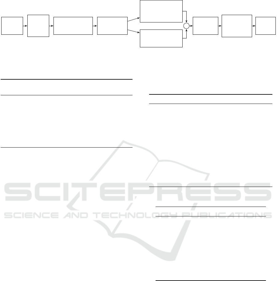
4.2 Feature Extraction

In order to remove high frequency noise, ﬁrst we ap-

ply a low pass ﬁlter to all the signals to smoothen the

Non-intrusive Distracted Driving Detection based on Driving Sensing Data

181

Driving

Signals

Low

Pass

Filter

Add 1

order

derivatives

Windowing

Function

PGP

SWA

All Signals

Extract

Statistical

Features

Extract Cepstral

Features

Classiﬁer

Decision

Function

or f

Output

ˆy

Figure 1: Distraction Detection Process.

Table 2: Selected Signals for Driver Identiﬁcation.

Sensor

order

Cepstral

Derivative

Percentage Gas Pedal (PGP) Yes Yes

Str. Wheel Angle (SWA) No Yes

Str. Wheel Rel. Speed (SWRS) No No

Vehicle Speed (VS) Yes No

Engine RPM (ERPM) Yes No

Pitch No No

Roll No No

Yaw No No

signals. Then for some of the signals (Shown in Table

2) we derive the temporal derivative of the signals.

For both smoothing and computation of derivations

we use an implementation of the Savitzky-Golay al-

gorithm (Savitzky, 1964). Figure 1 shows the vari-

ous stages that the signals go through before the fea-

ture extraction step. In this study we use 8 signals

which are listed in Table 2. These signals are obtained

from CAN-Bus or IMU. Then we apply a windowing

function to all the signals which takes two parame-

ters, w to determine the length of window frame and

r to specify amount of overlap between two consecu-

tive window frames. This will break down the sig-

nal into window frames of size w and is ready for

feature extraction stage. Per each signal, 9 statisti-

cal features are extracted from each window frame.

These descriptive statistics are selected to be repre-

sentative of the distribution of sensor values covered

by the window frame. This set includes minimum,

maximum, mean, median, standard deviation, kurto-

sis, skewness and number of zero crossings. We also

extract cepstral features from two signals, percent-

age of gas pedal (PGP) and SWA, these are the vehi-

cle operating inputs that are directly operated by the

driver. Earlier studies have proved that cepstral anal-

ysis are suitable for driver identiﬁcation (Jafarnejad

et al., 2017;

Ozt

urk and Erzin, 2012), we suspect that

they are also effective for detecting distracted driv-

ing. We compute the cepstral coefﬁcients similar to

Jafarnejad et al. and keep only the ﬁrst 32 coefﬁcients

and use as cepstral features (Jafarnejad et al., 2017).

4.3 Feature Importance

Table 3: Average Scores For Each Signal.

Signal Mutual Info. F-Test

SWRS 0.517 0.084

ERPM Derivative 0.510 0.059

Pitch 0.490 0.056

PGP Derivative 0.475 0.035

Roll 0.470 0.012

PGP 0.436 0.060

ERPM 0.428 0.359

VS Derivative 0.427 0.088

Yaw 0.425 0.054

VS 0.415 0.792

SWA 0.228 0.061

Cepstral Coefﬁcients PGP 0.029 0.036

Cepstral Coefﬁcients SWA 0.025 0.026

Table 4: Average Scores For Each Function.

Function Mutual Info. F-Test

Min 0.955 0.310

Max 0.933 0.289

Range 0.495 0.076

Median 0.136 0.309

Mean 0.092 0.314

Standard Deviation 0.053 0.067

# Zero crossings 0.040 0.166

Cepstral Coefﬁcients 0.034 0.039

Skewness 0.032 0.041

Kurtosis 0.030 0.081

We perform analysis on the extracted features to eval-

uate their ﬁtness for our experiments. We use two

metrics for this purpose, the conventional F-test and

Mutual Information (MI) as two metrics to evaluate

usefulness of our features as well as some insights

into which features or signals are more important for

our classiﬁcation task. To get an idea that which sig-

nal is more important, ﬁrst we compute the MI for all

features, we normalize it and compute the average for

5 best features from each signal. The corresponding

results are presented in Table 3. The signals are listed

in descending order of their MI. We do the similar

analysis for the statistical functions and cepstral coef-

ﬁcients, the corresponding results are presented in Ta-

VEHITS 2018 - 4th International Conference on Vehicle Technology and Intelligent Transport Systems

182

ble 4. Among the signals we can observe that features

extracted from steering wheel relative speed (SWRS)

have the highest MI score and the cepstral features

are the worst. In terms of functions used for feature

extraction we can see in Table 4 that very simple func-

tions such as Min, Max, Range, Mean are more useful

that Skewness and Kurtosis.

4.4 Classiﬁcation Algorithms

We select ﬁve classiﬁcation algorithms to be used as

window classiﬁer h

. The following is the list of clas-

siﬁers used in this study along with their correspond-

ing parameters.

• AdaBoost (AB) - 200 decision trees as weak

learners, learning rate = 0.75.

• Gradient Boosting (GB) 100 estimators, maxi-

mum depth = 6, maximum features = None, max-

imum depth = 6, learning rate = 0.05.

• Random Forest (RF) 200 estimators, maximum

features = None, maximum depth = 7, class

weight = balanced.

• K-Nearest Neighbors (KNN) # neighbors = 5.

• Support Vector Machine (SVM) RBF kernel, C

= 0.1, γ = 0.01.

For our experiments we use the scikit-learn software

package, all the other parameters are set to their

default values as of scikit-learn version 0.19.2 (Pe-

dregosa et al., 2011).

4.5 Decision Functions

The decision function f determines the ﬁnal predic-

tion ˆy at time t based on the last l window predictions,

we call this a decision window: h ˆy

t−l

,· ·· , ˆy

t−1

, ˆy

therefore l is the number of window frames covered

by a decision window. Below we introduce two de-

cision functions to obtain ˆy and evaluate their perfor-

mance later in Section 5:

1) Majority vote (MV) Let d to denote count of the

window frames in the decision window that are pre-

dicted as distracted driving. Then a decision window

is classiﬁed as distracted if

> 0.5.

2) Maximum score (MS) Let d

to be the cumulative

classiﬁcation score for distracted class. Then a deci-

sion window is classiﬁed as distracted if

> 0.5.

5 MODEL PERFORMANCE

In this section we present the results of our experi-

ments. In each subsection we focus on one of the

components of our proposed methodology and dis-

cuss their implications.

5.1 Sliding Window Analysis

In order to ﬁnd out the optimal sliding window size

we try various window sizes

as well as overlap ra-

tios

. Since we do not want to have our results inﬂu-

enced by the choice and working mechanism of the

decision function, in these experiments we do not ap-

ply the decision function f and only consider the pre-

dictions from h

. The results are presented in Fig-

ure 2, the reported numbers are the average cross val-

idated scores for each combination of r and w pa-

rameters. It is evident that results improve as over-

lap r increases. This can be explained by the fact

that an increase in overlap also increases the number

of window frames and therefore having more exam-

ples for the classiﬁer to learn from. It is also evi-

dent that performance improves as the window size

w increases, since our features are mostly descrip-

tive statistics, having larger window frames ﬁlters out

noise from the features therefore larger windows yield

better results. From this section we can conclude that

for both parameters r and w, it is best to choose a

larger value, however such choices have some draw-

backs as well. Larger values for r lead to increase in

number of examples and feature calculations, there-

fore becomes computationally more expensive. On

the other hand larger w results on longer delays in the

predictor, therefore w and r should be selected in a

manner suitable for application needs.

5.2 Classiﬁer Benchmarks

We run our experiments for all of the 5 selected clas-

siﬁers and compare their performance as h

, meaning

we only score the classiﬁers for their ability to pre-

dict individual window frames. Results are presented

in Figure 3 (obtained using w = 30s and r = 75%),

when considering ROC AUC score GB yields the best

performance and RF takes the second place.

We also investigate how different classiﬁers ex-

hibit different behaviors due to the changes of win-

dow size w. Figure 4 depicts the average cross val-

idated ROC AUC and F

scores for various window

sizes and ﬁxed overlap ratio of r = 75%. For example

KNN clearly beneﬁts from a larger window frame, be-

cause as it was discussed larger window frames result

in smoother features. On the contrary SVM does not

improve as much as other classiﬁers do, this may im-

Window sizes of 4, 7, 10, 15, 20, 30, 45 and 60

Overlap ratios of 0, 25, 50, 75 and 90 percent.

Non-intrusive Distracted Driving Detection based on Driving Sensing Data

183

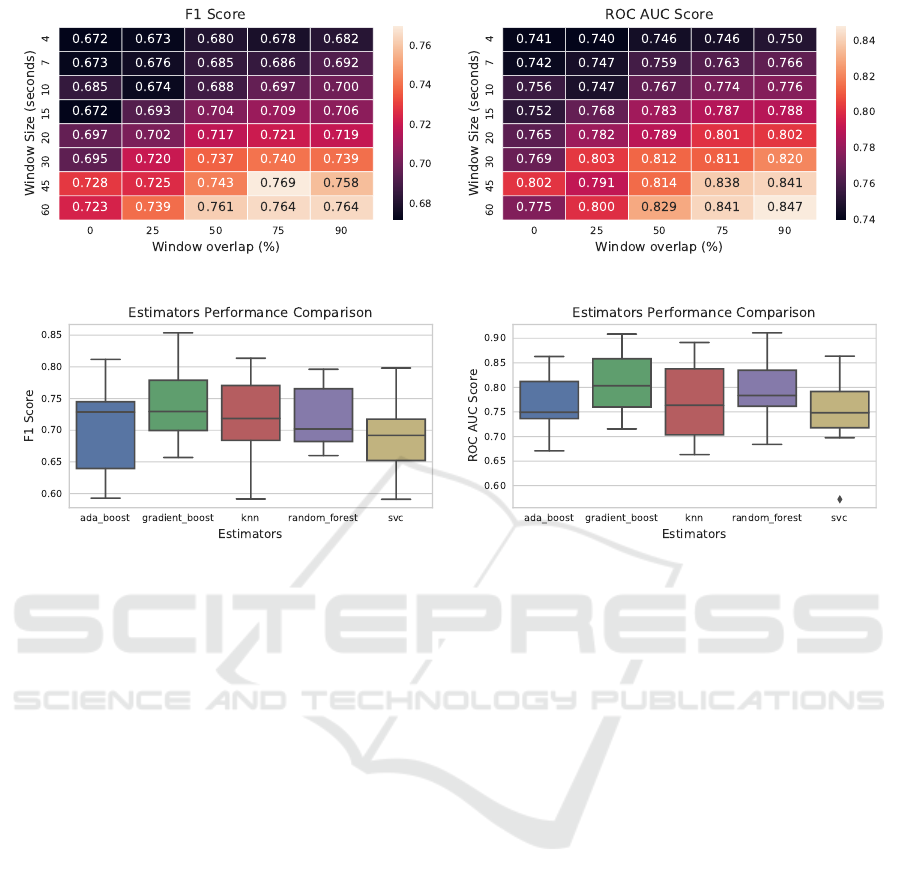
Figure 2: Effect of Window Size on Classiﬁcation Score.

Figure 3: Estimators Comparison - w = 30s and r = 75%.

prove by tuning the hyper-parameters for every win-

dow size however it is out of scope of this work.

5.3 Decision Function Benchmarks

Decision function f can be seen as a meta classi-

ﬁer which simply aggregates predictions from l con-

secutive window frames and outputs a single predic-

tion. We investigate its performance by running ex-

periments using values of 5, 10 and 15 for l and sim-

ilar combinations for w as previous experiments. To

compare the two proposed decision function a small

sample of results (Cases with DW Duration < 60s) is

presented in Table 5. The column DW Duration, in

the table refers to the timespan covered by the deci-

sion function f to make the prediction, these values

are computed considering overlap ratio of 75% be-

tween the consecutive window frames.

In order to demonstrate the advantage of using the de-

cision function, we also present the scores for individ-

ual window frame predictions, to have a fair compar-

ison for each row we compare the decision function

with the window frame conﬁgurations that is closest.

For example if w = 4s and DW Length = 15, DW Du-

ration will be 19 seconds, meaning the decision func-

tion effectively uses data from the past 19 seconds to

make a prediction. We compare this instance with the

predictions results for h

(classiﬁer without decision

function) with the w = 20s, because it is the closest

window frame size to 19s that we have considered. In

the table we can see that in f

results in between 4

to 9.3 % (6.6% in average) improvements over not us-

ing a decision function. f

performs worse than f

with average improvement of 3.58%.

6 DISCUSSION

If we consider how the data-set is annotated and the

signals we use for classiﬁcation it is expected not to be

able to achieve excellent results for detecting distrac-

tions. This is because we mark a long stretch of driv-

ing as distracted driving, however although in that pe-

riod driver is engaged in a certain secondary task, this

engagement is not uniformly present throughout the

stretch, therefore we are inadvertently injecting noise

into our training data. In fact one could perform the

labeling more granularly and potentially improve the

results. The proposed methodology is quite ﬂexible

and can be optimized for the intended applications,

generally one needs to ﬁnd the right balance between

the quality of detection and delay in detection. For

example using GB classiﬁer, w = 60, r = 0.75 and

DW = 15 (DW Duration of 285s) we achieve ROC

AUC of 98.7%. If we need a shorter the detection

time we get to ROC AUC of 92.7% with KNN clas-

VEHITS 2018 - 4th International Conference on Vehicle Technology and Intelligent Transport Systems

184

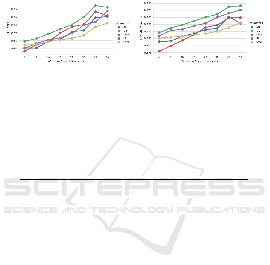
Figure 4: Estimators Performance Comparison - r = 75%.

Table 5: Decision Function Performance - Results are for KNN as classiﬁer.

Win. Decision Window (DW) Closest Window Decision Function

Len. (s) DW Len. DW Duration (s) Len. (s) ROC AUC ROC AUC MS ROC AUC MV

4 5 9.00 10 0.718 0.748 (+4.07) 0.718 (-0.09)

4 10 14.00 15 0.738 0.780 (+5.61) 0.759 (+2.80)

4 15 19.00 20 0.764 0.799 (+4.60) 0.782 (+2.34)

7 5 15.75 15 0.738 0.774 (+4.84) 0.751 (+1.74)

7 10 24.50 20 0.764 0.812 (+6.28) 0.799 (+4.57)

7 15 33.25 30 0.772 0.836 (+8.29) 0.825 (+6.92)

10 5 22.50 20 0.764 0.801 (+4.83) 0.760 (-0.58)

10 10 35.00 30 0.772 0.844 (+9.38) 0.814 (+5.44)

10 15 47.50 45 0.798 0.871 (+9.05) 0.846 (+5.89)

15 5 33.75 30 0.772 0.822 (+6.48) 0.802 (+3.89)

15 10 52.50 45 0.798 0.867 (+8.59) 0.855 (+7.09)

20 5 45.00 45 0.798 0.855 (+7.12) 0.822 (+2.96)

siﬁer, w = 20, r = 0.75 and DW = 15 (DW Duration

of 95s). For DW durations less than 60 seconds the

results are presented on Table 5, for smaller DW du-

rations, ROC AUC decreases. We should also point

out that our evaluations are done not knowing any-

thing about the individual, in other words the model is

always trained on drivers that are not among the test

set. Tango and Botta (Tango and Botta, 2013) indi-

cate that they have gained about 20% improvement in

the performance when they trained a model for each

driver (Intra-subject). Another important factor is that

we do not use any intrusive signals, not tracking of the

driver’s head nor the cabin sound, only sensor data

from the car. Not only that, studies such as (W

ollmer

et al., 2011) and (Tango and Botta, 2013) regardless

of intrusive sensors, they do use metrics that are not

readily available. Such as distance from the center of

the lane. Such information are one of the key metrics

inﬂuenced by the distracted driving. However here

our goal is to make a similar prediction without hav-

ing access to such information. With the current setup

we may not be able to address applications that re-

quire accurate spontaneous and momentarily distrac-

tion detection. Instead the system performs well at

detecting long lasting distractions, such as mobile-

phone conversations or conversations among the pas-

sengers. Moreover one can use such a system as a

way to characterize driver’s riskiness. It is crucial for

insurance, logistic and public transport companies, to

keep track of their customers or employees risky driv-

ing behavior. Such application is equally beneﬁcial

for individuals who would like to keep track of their

driving quality. For example parents who are con-

cerned about safety of their teenagers, would like to

know whether or not their children is a risky driver.

7 CONCLUSIONS

In this paper, we have proposed a mechanism to de-

tect distracted driving based on non-intrusive vehicle

sensor data. In the proposed method 8 driving signals

are used. The data is collected, two types of statistical

and cepstral features are extracted in a sliding win-

dow process, next a classiﬁer makes a prediction for

each window frame, and lastly, a decision function

takes the last l predictions and makes the ﬁnal pre-

diction for the given window frames. We have evalu-

ated the subject independent performance of the pro-

posed mechanism using a driving data-set consisting

of 13 drivers. We analyzed the implications of chang-

ing the size of sliding window and its overlap ratio.

We have shown that the performance increases as the

window size and decision window size become larger.

Non-intrusive Distracted Driving Detection based on Driving Sensing Data

185

We have compared the performance of several classi-

ﬁers. The best results were achieved using GB classi-

ﬁer w = 60,r = 0.75 and DW = 15 (DW Duration of

285s) which yields ROC AUC of 98.7%. Our results

show that even with poorly annotated data and only

use of vehicle sensor data it is possible to accurately

detect distracted driving events. In future work intra-

subject models should be evaluated. It will be also of

interest to see how the proposed mechanism performs

on a more granular dataset, with more accurate labels.

ACKNOWLEDGEMENTS

The authors would like to thank Dr. H

useyn Abut

and VPALAB of Sabanci University for providing the

data-set used for this study.

REFERENCES

Abut, H., Erdo

gan, H., Erc¸il, A., C¸

ukl

u, A. B., Koman,

H. C., Tas, F., Arguns¸ah, A.

O., Akan, B., Karabalkan,

H., C¸

okelek, E., et al. (2007). Data collection with”

uyanik”: too much pain; but gains are coming.

Berka, C., Levendowski, D. J., Lumicao, M. N., Yau,

A., Davis, G., Zivkovic, V. T., Olmstead, R. E.,

Tremoulet, P. D., and Craven, P. L. (2007). EEG Cor-

relates of Task Engagement and Mental Workload in

Vigilance, Learning, and Memory Tasks.

Dietterich, T. G. (2002). Machine learning for sequential

data: A review. In Joint IAPR International Work-

shops on Statistical Techniques in Pattern Recognition

(SPR) and Structural and Syntactic Pattern Recogni-

tion (SSPR), pages 15–30. Springer.

Dong, Y., Hu, Z., Uchimura, K., and Murayama, N. (2011).

Driver inattention monitoring system for intelligent

vehicles: A review. IEEE Transactions on Intelligent

Transportation Systems, 12(2):596–614.

Engstr

om, J., Monk, C. A., Hanowski, R. J., Horrey, W. J.,

Lee, J. D., McGehee, D. V., Regan, M. a., Stevens, A.,

Traube, E., Tuukkanen, M., Victor, T., and Yang, D.

(2013). A Conceptual Framework and Taxonomy for

Understanding and Categorizing Driver Inattention.

Farneb

ack, G. (2003). Two-Frame Motion Estimation

Based on Polynomial Expansion. Springer.

Fridman, L., Brown, D. E., Angell, W., Abdi

c, I., Reimer,

B., and Noh, H. Y. (2016). Automated synchro-

nization of driving data using vibration and steering

events. Pattern Recogn. Lett., 75(C):9–15.

Harbluk, J. L., Noy, Y. I., Trbovich, P. L., and Eizenman, M.

(2007). An on-road assessment of cognitive distrac-

tion: Impacts on drivers’ visual behavior and brak-

ing performance. Accident Analysis and Prevention,

39(2):372–379.

Jafarnejad, S., Castignani, G., and Engel, T. (2017). To-

wards a real-time driver identiﬁcation mechanism

based on driving sensing data. In 20th Interna-

tional Conference on Intelligent Transportation Sys-

tems (ITSC). IEEE.

Jin, L., Niu, Q., Hou, H., Xian, H., Wang, Y., and Shi, D.

(2012). Driver cognitive distraction detection using

driving performance measures. Discrete Dynamics in

Nature and Society.

Klauer, S. G., Guo, F., Sudweeks, J., and Dingus, T. A.

(2010). An analysis of driver inattention using a case-

crossover approach on 100-car data. Technical report.

Lee, J., Young, K., and Regan, M. (2009). Deﬁning driver

distraction, pages 31 – 40. CRC Press, Australia.

Liang, Y. and Lee, J. D. (2010). Combining cognitive and

visual distraction: Less than the sum of its parts. Ac-

cident Analysis and Prevention, 42(3):881–890.

Miyajima, C., Kusakawa, T., Nishino, T., Kitaoka, N., Itou,

K., and Takeda, K. (2009). On-going data collection

of driving behavior signals. In In-Vehicle Corpus and

Signal Processing for Driver Behavior. Springer.

Ozt

urk, E. and Erzin, E. (2012). Driver Status Identiﬁcation

from Driving Behavior Signals, pages 31–55. Springer

NY, New York, NY.

Pedregosa, F., Varoquaux, G., Gramfort, A., Michel, V.,

Thirion, B., Grisel, O., Blondel, M., Prettenhofer,

P., Weiss, R., Dubourg, V., Vanderplas, J., Passos,

A., Cournapeau, D., Brucher, M., Perrot, M., and

Duchesnay, E. (2011). Scikit-learn: Machine learning

in Python. Journal of Machine Learning Research,

12:2825–2830.

Rantanen, E. M. and Goldberg, J. H. (1999). The effect

of mental workload on the visual ﬁeld size and shape.

Ergonomics, 42(6):816–834.

Savitzky, A. Golay, M. J. E. (1964). Smoothing and dif-

ferentiation of data by simpliﬁed least squares proce-

dures. Anal. Chem., 36.

Tango, F. and Botta, M. (2013). Real-time detection system

of driver distraction using machine learning. IEEE

Transactions on Intelligent Transportation Systems,

14(2):894–905.

Wesley, A., Hoffman Hall, P. G., Shastri, D., and Pavlidis,

I. (2010). A Novel Method to Monitor Driver’s Dis-

tractions CHI 2010: Work-in-Progress.

ollmer, M., Blaschke, C., Schindl, T., Schuller, B.,

arber, B., Mayer, S., and Trefﬂich, B. (2011). Online

Driver Distraction Detection Using Long Short-Term

Memory. IEEE Transactions on Intelligent Trans-

portation Systems, 12(2).

Zhou, H., Itoh, M., and Inagaki, T. (2008). Inﬂuence of cog-

nitively distracting activity on driver’s eye movement

during preparation of changing lanes. Proceedings of

the SICE Annual Conference, pages 866–871.

VEHITS 2018 - 4th International Conference on Vehicle Technology and Intelligent Transport Systems

186