Optimal Estimation of Census Block Group Clusters to Improve the

Computational Efﬁciency of Drive Time Calculations

Damon Gwinn

, Jordan Helmick

, Natasha Kholgade Banerjee

and Sean Banerjee

Clarkson University, Potsdam, NY, U.S.A.

MedExpress, Morgantown, WV, U.S.A.

Keywords:

Location Selection, Census Block Group, Afﬁnity Propagation.

Abstract:

Location selection determines the feasibility of a new location by evaluating factors such as the drive time

of customers, the number of potential customers, and the number and proximity of competitors to the new

location. Traditional location selection approaches use census block group data to determine average customer

drive times by computing the drive time from each block group to the proposed location and comparing it

to all competitors within the area. However, since companies need to evaluate on the order of hundreds

of thousands of potential locations and competitors, traditional location selection approaches prove to be

computationally infeasible. In this paper we present an approach that generates an optimal set of clusters to

speed up drive time calculations. Our approach is based on the insight that in urban areas block groups are

comprised of a few adjacent city blocks, making the differences in drive times between neighboring block

groups negligible. We use afﬁnity propagation to initially cluster the census block groups. We use population

and average distance between the cluster centroid and all points to recursively re-cluster the initial clusters. Our

approach reduces the census data for the United States by 80% which provides a 5× speed when computing

drive times. We sample 200 randomly generated locations across the United States and show that there is

no statistically signiﬁcant difference in the drive times when using the raw census data and our recursively

clustered data. Additionally, for further validation we select 300 random Walmart stores across the United

States and show that there is no statistically signiﬁcant difference in the drive times.

1 INTRODUCTION

Location selection determines the feasibility of a new

retail location by evaluating factors such as the drive

time of customers to the new location, the number of

potential customers, and the number and proximity of

competitors to the new location. Locations that are

distant from the customer base, out-positioned by a

major competitor, or in a rural area with a low pop-

ulation density are less likely to succeed. Drive time

computations for a new location are performed by us-

ing the census block group data in conjunction with

drive time analysis tools, such as the Google Maps

Distance Matrix API (Google, 2017). For a pro-

posed location, a trade area is created around the lo-

cation and drive times are computed from each block

group within the trade area to the proposed location.

The drive times are then averaged and compared with

competing locations to determine if the proposed lo-

cation is closer than the competition.

However, since companies need to evaluate on the

order of thousands of potential locations and competi-

tors, computing drive times from each census block

group can be computationally infeasible. In this pa-

per, we present an approach to reduce the computa-

tional overhead for drive time calculations by cluster-

ing neighboring block groups into a single point. Our

insight is that census block groups in urban areas are

in close proximity, as shown in Figure 1, making drive

time calculations from each block group redundant as

the differences in driving time between neighboring

block groups are negligible.

In this paper we present an approach to estimate

an optimal set of census block group clusters. The

novelty of our approach is a recursive algorithm to

split large clusters into optimal-sized clusters that

satisfy user-provided thresholds of population count

and average distance between the cluster centroid and

cluster members. We ﬁrst generate an initial set of

clusters using afﬁnity propagation (Frey and Dueck,

2007) which automatically estimates the number of

clusters for an input set of points. We recursively

Gwinn, D., Helmick, J., Kholgade Banerjee, N. and Banerjee, S.

Optimal Estimation of Census Block Group Clusters to Improve the Computational Efﬁciency of Drive Time Calculations.

DOI: 10.5220/0006707800960106

In Proceedings of the 4th International Conference on Geographical Information Systems Theory, Applications and Management (GISTAM 2018), pages 96-106

ISBN: 978-989-758-294-3

Figure 1: Two neighboring census block groups in Wash-

ington, DC. As shown by the Google Maps distance and

drive time calculation, the block groups are 0.2 miles which

equates to a 1 minute driving time. The difference in dis-

tance and drive time is insigniﬁcant and the block groups

can be clustered to a single point. In this paper, we leverage

block group proximity to cluster neighboring block groups

into a single point to reduce computational overhead.

split clusters if their human population count or av-

erage distance from each member to the cluster cen-

troid are higher than user-provided thresholds, and if

there are more than 10 block groups in each cluster.

We approximate the distances between each cluster

member and the cluster centroid by using the haver-

sine formula (Van Brummelen, 2012).

The remainder of this paper is organized as fol-

lows: in Section 2 we discuss the related literature in

location selection. Section 3 discusses our recursive

threshold based cluster splitting approach. In Sec-

tion 4 describe our dataset, and we show the com-

putational improvements gained by clustering block

groups. We discuss the practical and statistical dif-

ferences in drive times using 200 random locations in

Section 5. We discuss internal and external validity

threats in Section 6. Finally, we conclude the paper in

Section 7 and provide potential directions for future

research.

2 RELATED WORK

Several approaches use a variety of features extracted

from the data in location selection. The approach of

Xu et al. (Xu et al., 2016) features such as distances

to the city center, trafﬁc, POI density, category pop-

ularity, competition, area popularity, and local real

estate pricing to determine the feasibility of a loca-

tion. The approach of Karamshuk et al. (Karamshuk

et al., 2013) uses features mined from FourSquare

along with supervised learning approaches using Sup-

port Vector Regression, M5 decision trees, and Linear

Regression to determine the optimal location of a re-

tail store.

Social media platforms provide novel metrics to

evaluate the feasibility of a location. Several ap-

proaches determine the popularity of a proposed lo-

cation by using the reviews of users (Wang et al.,

2016a), or by evaluating the number of user check-

ins and location centric data from platforms such as

Twitter and FourSquare (Karamshuk et al., 2013; Qu

and Zhang, 2013; Yu et al., 2013; Yu et al., 2016;

Wang et al., 2016b; Chen et al., 2015). User com-

ments posted on review sites provide insights on the

personal experience of the consumer at an existing lo-

cation or similar business. User check-in data pro-

vides popularity metrics for a geographical area based

on the frequency and duration of a visit.

Many approaches use optimal location queries

to evaluate the effectiveness of a location by plac-

ing higher priority on locations that are closer to

the proposed customer base (Xiao et al., 2011;

Ghaemi et al., 2010). The approach of Ghaemi et

al. (Ghaemi et al., 2012) uses nearest neighbors with

results from past optimal location queries to address

issues caused by moving locations and customers.

Banaei et al. (Banaei-Kashani et al., 2014) propose re-

verse skyline queries to allow optimal location queries

to handle multiple criteria such as distance to location

and distance to competitors.

Since a proposed location may not satisfy all cri-

teria adequately, Kahraman et al. (Kahraman et al.,

2003) use fuzzy techniques to reach a compromise be-

tween various criteria while evaluating the feasibility

of a site. Fuzzy approaches have been used to de-

termine the appropriate number of ﬁrestations at an

airport (Tzeng and Chen, 1999), and the optimal lo-

cation of new convenience stores (Kuo et al., 1999)

and factories (C¸ ebi and Otay, 2015; Yong, 2006). Ap-

proaches based on analytic hierarchy process (AHP)

use human experts to weight location selection crite-

ria and to generate a comprised location rank (Tzeng

et al., 2002; Yang and Lee, 1997; Aras et al., 2004).

Unlike the prior approaches, our work uses cen-

sus block group data, and is most closely related to

research in the area of retail location selection, ser-

vice accessibility and market demands using census

block groups (Bailey, 2003; Nallamothu et al., 2006;

Carr et al., 2009; Guagliardo, 2004; Jiao et al., 2012;

Branas et al., 2005; Farber et al., 2014; Blanchard and

Lyson, 2002). Several approaches use census block

groups and tracts to compute population and drive

time estimates for access to trauma centers, hospitals,

grocery stores, and supermarkets (Branas et al., 2005;

Nallamothu et al., 2006; Carr et al., 2009; Guagliardo,

2004; Jiao et al., 2012; Farber et al., 2014; Blanchard

and Lyson, 2002). Unlike our work, these approaches

estimate drive times by using urban, suburban, and

rural speed thresholds and population densities. In

the absence of accurate drive time data for location

Optimal Estimation of Census Block Group Clusters to Improve the Computational Efﬁciency of Drive Time Calculations

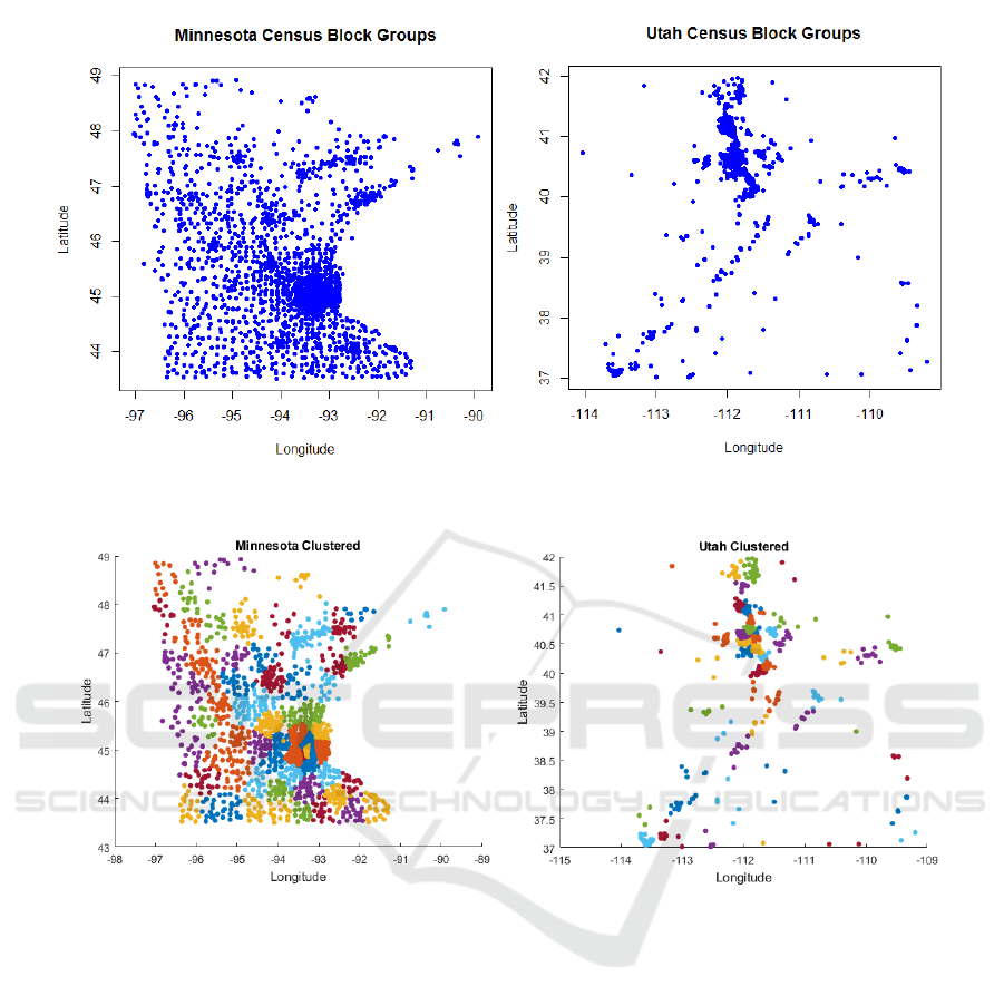
Figure 2: Comparison of census block group distribution for Minnesota and Utah. While both states are approximately 85,000

square miles, Utah has large uninhabited areas when compared to Minnesota.

Figure 3: Comparison of clustered census block groups for Minnesota and Utah. While both states have the same land area,

Utah has only 51 clusters while Minnesota has 134 clusters. Hence, traditional clustering approaches cannot be applied as

we have no prior knowledge of the number of optimal clusters. In our approach we use afﬁnity propagation, which does not

assume a base number of optimal clusters.

selection, the approach of Li et al. (Li et al., 2015)

computes road segment times from public transit GPS

data. Our work differs from these approaches in

that all these approaches use unclustered census block

groups and drive time estimates for evaluating the fea-

sibility of a proposed location. Unclustered census

data introduces computational overhead when select-

ing across multiple candidate locations and compar-

ing to multiple competitors. Drive time estimates do

not accurately depict the time taken by customers to

reach the location. Instead we propose using exact

drive times obtained from Google Maps, while using

clustering to reduce computational overhead.

3 THRESHOLD BASED

RECURSIVE CLUSTERING

3.1 Base Clustering Algorithm

We use afﬁnity propagation as our base clustering al-

gorithm as it does not require the user to specify the

number of clusters (Frey and Dueck, 2007). In our

case, we have no prior knowledge on the optimal clus-

ter size. Further, each state can have a different num-

ber of clusters based on the population distribution.

For example, as shown in Figure 2, Utah and Min-

nesota have the same overall land area, but have dif-

ferent census block group distributions due to their

GISTAM 2018 - 4th International Conference on Geographical Information Systems Theory, Applications and Management

geography. As shown in Figure 3, Utah has 51 clus-

ters while Minnesota has 134 clusters. Densely popu-

lated areas are combined into multiple clusters, while

sparsely populated areas are combined into a single

cluster. Minnesota has several densely populated ar-

eas, and hence requires a larger number of clusters to

describe the state.

We use the afﬁnity propagation algorithm im-

plemented in the Python skikit-learn toolkit using

2000 maximum iterations and 200 convergence iter-

ations (Pedregosa et al., 2011). The convergence it-

erations control the number of iterations without any

changes in the estimated clusters. A high maximum

and convergence iteration provides higher certainty

that the resultant clusters will not change.

3.2 Recursive Cluster Splitting

Our recursive cluster splitting method uses the initial

clusters generated in Subsection 3.1, a user-provided

upper bound

bound

for the mean distance between the

cluster centroid and each cluster point, and a user-

provided upper bound p

bound

for the total population

in each cluster as input. For the results shown in this

paper, we set d

bound

to 5 and p

bound

to 20, 000. For

each cluster c from Subsection 3.1, we compute the

distance d

between the cluster centroid and the i

point in the cluster, where i ∈ I

and I

represents the

indices of all points in the c

cluster, as

= R ·b

, (1)

where b

is given by

= 2atan2



√

1 −a



. (2)

The value of a

represents the haversine of the central

angle between each point represented by its latitude

and longitude λ

to its cluster centroid represented

by φ

and λ

, and is computed as

= sin

−φ

+ cos φ

·cos φ

·sin

−λ

. (3)

In Equation (1), R represents the radius of the earth at

the equator, i.e., 3959 miles. For cluster c, we com-

pute the mean distance

d for all points in the cluster

to its centroid as

d =

∑

i∈I

. (4)

We split cluster c into a second set of clusters us-

ing afﬁnity propagation if

d is higher than the user-

speciﬁed upper bound

bound

or the population in the

cluster p

is higher than p

bound

, and if the num-

ber of points in a cluster is greater than 10. For each

Algorithm 1: Recursive Cluster Splitting.

Input: Sets of latitudes and longitudes for

initial cluster points

{{(φ

, λ

) : i ∈I

init

} : c

init

∈ C

init

Set of latitudes and longitudes for initial cluster

centroids {(φ

init

, λ

init

: c

init

∈ C

init

}, and

user-provided bounds

bound

and p

bound

Output: Set of ﬁnal clusters, O

1 for c

init

∈ C

init

2 P

init

← {(φ

, λ

) : i ∈I

init

}

3 O = split(P

init

,O)

4 return O

end

Procedure split(P

,O)

1 Compute

using Equation (4)

2 if (

bound

∨p

> p

bound

) ∧

> 10

then

3 Split cluster represented by points in P

by clustering them into smaller

clusters {P

¯c

: ¯c ∈ C

} using afﬁnity

propagation

4 for ¯c ∈ C

5 return split(P

¯c

,O)

end

else

6 O ← O ∪P

7 return O

end

newly generated cluster, we recursively perform av-

erage distance computation and evaluation of the dis-

tance, population, and cluster point count to split them

further till the user-deﬁned constraints are met. Algo-

rithm 1 summarizes the steps of our approach. The

initial clustering algorithm runs in O(kn

) time and

produces R clusters, where k represents the number

of iterations until convergence and n represents the

number of samples. In our case, the initial clustering

algorithm runs with n = 220,334 points and k = 200.

Each of the R clusters is reclustered in O(km

) time,

where k = 200 and m

represents the number of points

in the i

cluster and i ∈ R.

3.3 Drive Times Computation

When evaluating the effectiveness of our approach,

we compute exact drive times to a potential location

from all points enclosed by a bounding box at a user

speciﬁed distance (e.g. 5 miles). The bounding box is

represented by coordinates of the north east and south

west most points. All points within the bounding box

are clustered census block groups generated by Al-

Optimal Estimation of Census Block Group Clusters to Improve the Computational Efﬁciency of Drive Time Calculations

Algorithm 2: Bounding Box Computation.

Parameters: MINLAT (min latitude):−90

◦

MAXLAT (max latitude):90

◦

MINLON (min

longitude):−180

◦

MAXLON (max longitude):180

◦

R (radius of earth): 6, 371 km.

Input: Distance d and location (φ

,λ

)

1 φ =

2 φ

min

= φ

−φ

3 φ

max

= φ

+ φ

4 if φ

min

> MINLAT ∧φ

max

< MAXLAT then

5 λ = sin

−1



sinφ

cosφ



6 λ

min

← λ

−λ

7 if λ

min

< MINLON then

8 λ

min

← λ

min

+ 2π

end

9 λ

max

← λ

+ λ

10 if λ

max

> MAXLON then

11 λ

max

← λ

max

−2π

end

else

12 φ

min

← max(φ

min

, MINLAT)

13 φ

max

← min(φ

max

, MAXLAT)

14 λ

min

← MINLON

15 λ

max

← MAXLON

end

Figure 4: We use the drive times generated by the Google

Maps API to determine the differences between raw census

block group data and our recursively clustered data. The

JSON object payload contains distance and drive time val-

ues from a given starting and ending location.

gorithm 1, and represent customers who are likely to

visit the potential location. We compute the locations

of the north east and south west most points of the

bounding box by using the inverse haversine formula

described in Algorithm 2. Given a distance d and the

location denoted with latitude φ

and longitude λ

we compute the north east location with latitude φ

max

and longitude λ

max

and the south west location with

latitude φ

min

and longitude λ

min

. We use the Google

Maps API to generate drive times for all points en-

closed by bounding box to the location. For exam-

ple, to compute the drive time and distance between

starting location (44.66, -74.99) and ending location

(44.67, -74.98), we call the mapping API using: ht

tp://map s.googleapis.c om/maps/api/di stanc

ematrix/ json?units=imp erial&origins= 44.66

,-74.99&destinations=44.67,-74.98. The re-

turned JSON object is shown in Figure 4. The gener-

ation of the north east and south west most points of

the bounding box are performed in O(1) time, while

the drive time computations are performed in O(n)

time, where n represents the number of points within

the bounding box.

4 RESULTS

We use the 2010 US Census Bureau Block

Group dataset which consists of 220,334 unique

block groups representing all 50 states, District of

Columbia, and Puerto Rico (Census, 2010). The

dataset consists of:

• STATEFP or State Federal Information Process-

ing Standards (FIPS) code, which is used to iden-

tify each state in the US,

• COUNTYFP or county FIPS code, which is used

to identify each county within the state,

• POPULATION or the total population of the

block group,

• LATITUDE or the latitude of the block group cen-

ter, and

• LONGITUDE or the longitude of the block group

center.

Our approach reduces the size of the census

dataset from 220,334 block groups to 41,442 clus-

tered block groups, thereby reducing the dataset by

81.19%. On a per state basis, we see the highest re-

duction in Rhode Island, with a reduction from 815

block groups to 117 clusters resulting in a reduction

of 85.64%. We see the lowest reduction in North

Dakota, with a reduction from 572 block groups to

164 clusters, or a reduction of 71.33%.

The average maximum distance from the cluster

centroid across all states is 4.624 miles. The aver-

age distance from the cluster centroid to cluster points

across all states is 2.300 miles. On a per state basis,

we see the lowest average maximum distance from

GISTAM 2018 - 4th International Conference on Geographical Information Systems Theory, Applications and Management

100

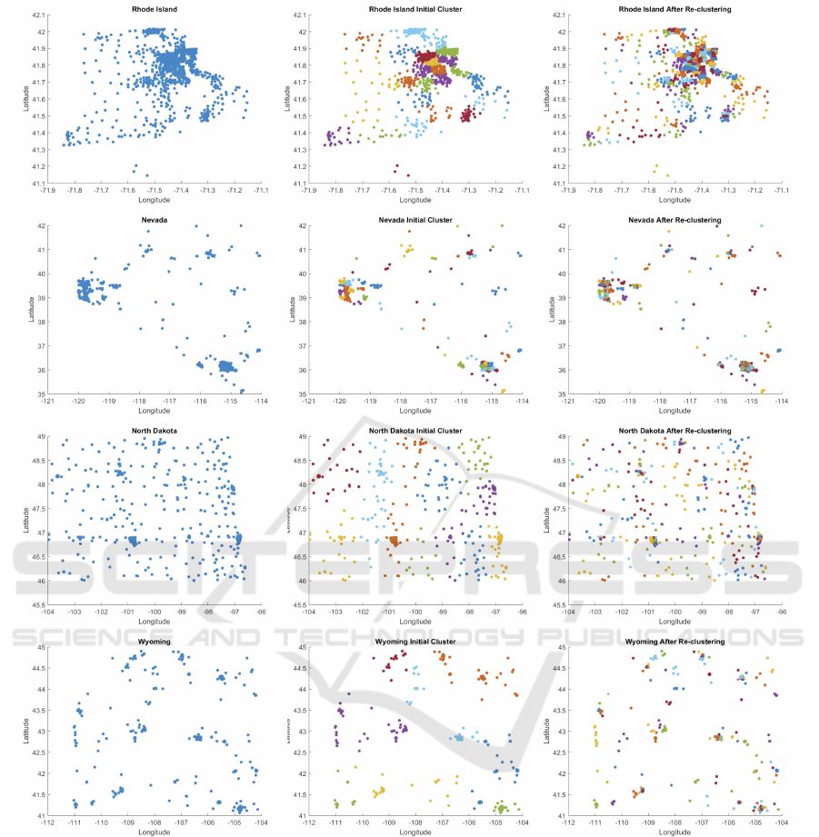
Figure 5: Comparing results for raw census block group data, sub-optimal clustered data, and optimally clustered data for

Rhode Island, Nevada, North Dakota, and Wyoming. A densely populated state, such as Rhode Island, or a state with dense

population localities, can be described by fewer clusters. Sparsely populated states, such as North Dakota and Wyoming,

require a larger number of clusters to deﬁne the population. (Figure best viewed in color).

the cluster centroid in the District of Columbia at

0.667 miles. The lowest average distance from the

cluster centroid to cluster points is also in the District

of Columbia at 0.381 miles. We see the highest av-

erage maximum distance from the cluster centroid in

Alaska at 27.141 miles. The highest average distance

from the cluster centroid to cluster points is also in

Alaska at 11.369 miles. For a congested state with

dense trafﬁc patterns and low inner city speed limits,

such as the District of Columbia, a low cluster cen-

troid to cluster point distance is ideal. On the other

hand, for a sparsely populated state, such as Alaska,

where speed limits are higher a larger cluster centroid

to cluster point distance has minimal impact.

The state to state variations in census block group

reduction can be explained by the differences in land

area and population distribution. As shown in Fig-

ure 5 census block group reduction is highest in

Rhode Island as it is a densely populated state with

1021 individuals per square mile. States such as

Optimal Estimation of Census Block Group Clusters to Improve the Computational Efﬁciency of Drive Time Calculations

101

Figure 6: A densely populated area contains several block groups in close proximity, while a sparesely populated area has

larger distances between block groups. In our approach the densely populated area shown in the top right is reclustered further

into smaller clusters to ensure each cluster point is less than 5 miles from the cluster centroid and the total population of the

cluster is below 20,000. The sparsely populated area shown on the bottom right will also be reclustered using our approach,

however our algorithm generates fewer sub clusters. (Figure best viewed in color).

Nevada, where the population density is low (26 in-

dividuals per square mile), but highly concentrated to

a few localities also have a higher reduction (84.80%).

On the other hand, states with a low population den-

sity, such as Wyoming with 6 individuals per square

mile have the lowest reduction.

For a densely populated state, such as Rhode Is-

land, we start with 815 census block groups and gen-

erate a set of 27 sub-optimal clusters. These initial

clusters are sub-optimal as the average maximum dis-

tance from the cluster centroid of 6.825 miles and an

average cluster centroid to cluster points distance of

3.272 miles. Using our approach, we generate 117

optimized clusters. The average maximum distance

from the cluster centroid is 2.285 miles, and the aver-

age distance from the cluster centroid to cluster points

is 1.259 miles. On the other hand, for a sparsely

populated state, such as South Dakota, we start with

654 census block groups and generate a set of 15

sub-optimal clusters. The average maximum distance

in the sub-optimal clusters is 76.994 miles and the

average cluster centroid to cluster points distance is

30.607 miles. Our approach generate 177 optimized

clusters with a average maximum distance of 8.501

miles and an average cluster centroid to cluster points

distance of 4.264 miles.

To understand how localities with different popu-

lation densities are handled by our approach, we show

the changes in cluster distribution after initial clus-

ter and optimization for two localities in Connecticut

in Figures 6 and 7. As shown in Figure 7, after ini-

tial clustering a densely populated areas, such as the

Hartford area, has a large number of block groups in

close spatial proximity. A sparsely populated area,

such as the Salisbury area has very few census block

groups with a larger distance between neighboring

block groups. As shown in Figure 7, after optimiza-

tion our approach generates clusters comprised of 10

or more census block groups in densely populated

areas since the distance between cluster members is

low. For sparsely populated areas, each cluster con-

sists of 3-4 census block groups as they are spatially

further apart from each other.

The 80% reduction in the census dataset results

in a 5× increase in computational efﬁciency on aver-

age. As shown in Figure 8 for our random location

denoted by the diamond symbol and located at coor-

dinates (41.766458,-72.677643), we generate 253 po-

tential customers groups in a 5 mile bounding box us-

ing the census block group data with an average drive

time of 10 minutes 14 seconds. Our approach gen-

erates 33 clustered customer groups with an average

drive time of 10 minutes 5 seconds.

GISTAM 2018 - 4th International Conference on Geographical Information Systems Theory, Applications and Management

102

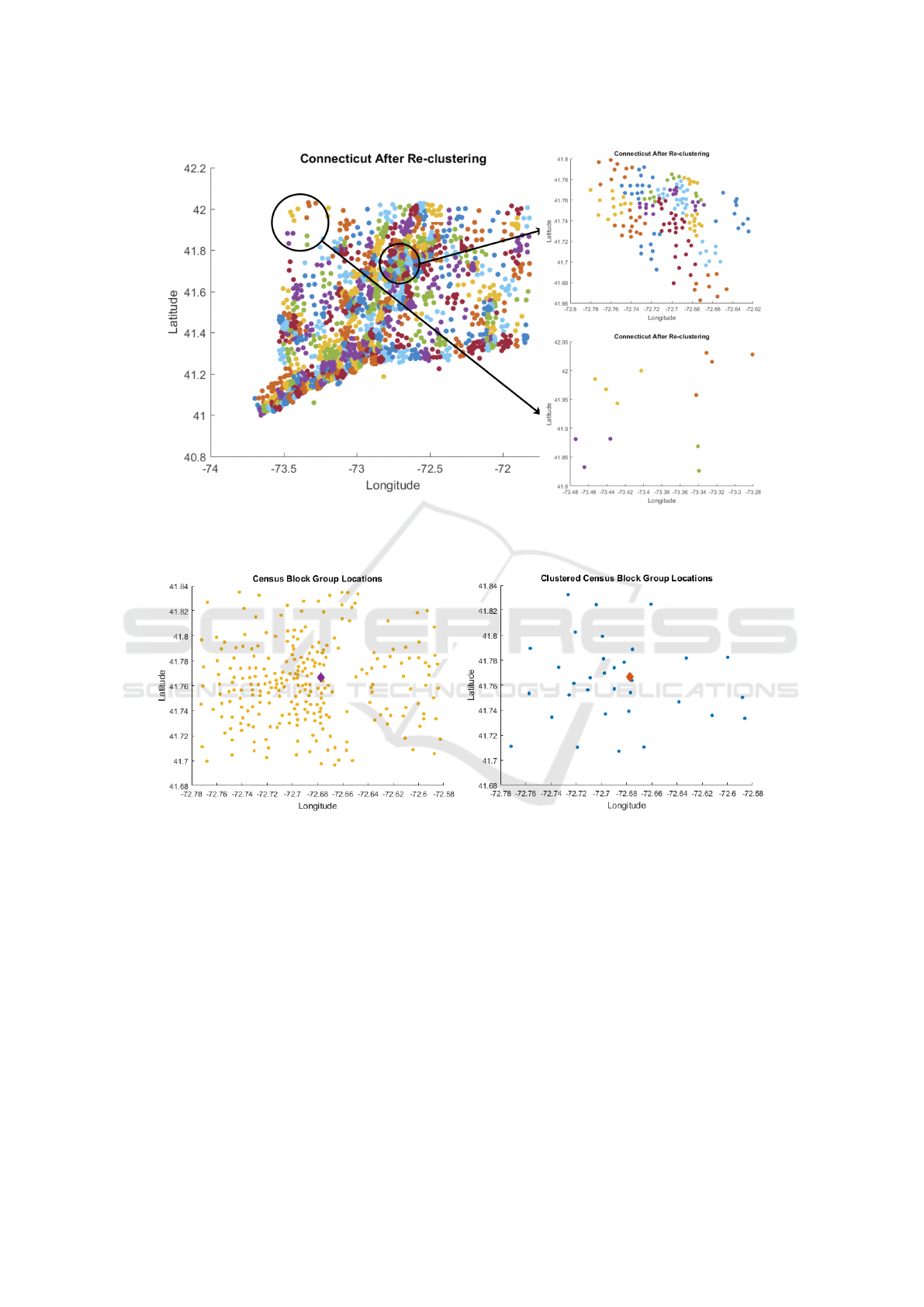
Figure 7: A densely populated area contains several block groups in close proximity, while a sparsely populated area has

larger distances between block groups. By reclustering the densely populated area into multiple smalller clusters, we ensure

that the drive time differences between the raw census data and clustered data are minimized. (Figure best viewed in color.)

Figure 8: Effect of clustering on reducing the number of drive time computations in a urban location, such as Hartfod, CT.

The diamond indicates a proposed location, and the circles indicate block groups. The ﬁgure on the left shows the raw census

block group data, while the ﬁgure on the right shows the clustered block group data.

5 EVALUATION

The typical location selection process involves the

evaluation of drive times for several thousand loca-

tions across the country and making comparisons to

several thousand competitors. We measure the perfor-

mance of our optimized clustering approach by com-

puting the difference in drive times for 200 random

locations generated across the entire US. For each lo-

cation we create a trade area at a radius of 5 miles

from the location and compute the average drive time

using both the census block group data and the opti-

mally clustered data. We apply a paired t-test and test

the following hypotheses:

NULL : the mean drive time for census block

group data is no different from the mean drive time

for optimally clustered data.

Alternate : the mean drive time for census block

group data is different from the mean drive time for

optimally clustered data.

We failed to reject the NULL hypothesis with a

p-value of 0.1878. The difference in sample means

for the census block group data and clustered data is

0.224301 minutes or 13.5 seconds. The 95% conﬁ-

Optimal Estimation of Census Block Group Clusters to Improve the Computational Efﬁciency of Drive Time Calculations

103

dence interval lies between [-33.53 seconds, 6.62 sec-

onds]. For the census block group data, we compute

drive times to 8855 consumer groups. By using the

clustered census block groups we only compute drive

times to 1570 locations, resulting in a 5.64×improve-

ment in the number of computations.

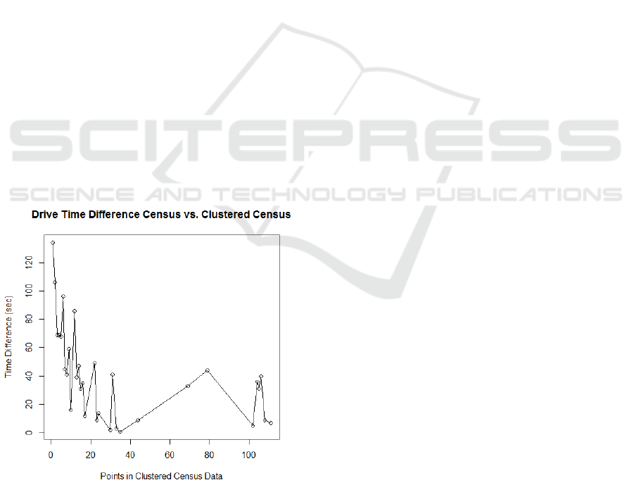
The differences in drive times obtained from the

census and clustered census data are impacted by

the number of clustered points found within a trade

area for a proposed location. As shown in Figure 9,

sparsely populated areas where the clustering reduces

to the census block groups to 1 or 2 clusters results

in a higher difference in drive times. In sparse ar-

eas, we observe drive time differences up to 2 minutes

on average when comparing the census and clustered

census data. For densely populated areas, where cen-

sus block groups are in close spatial proximity, the

drive time differences are less than 30 seconds on av-

erage. A 2 minute drive time difference in a sparsely

populated area, where amenities are in general further

apart, may be more acceptable to a consumer.

To further validate our approach, we randomly se-

lected 300 Walmart locations and computed the drive

time using our optimized clustering approach and the

raw census data. We failed to reject the NULL hy-

pothesis with a p-value of 0.08782. The difference in

sample means for the census block group data and the

clustered data is 0.1464922 minutes or 8.8 seconds.

The 95% conﬁdence interval lies between [-18.89 sec-

onds, 1.31 seconds].

Figure 9: Drive time differences measured in seconds for

census vs. clustered census data. Drive time differences re-

duce as the number of clustered points in the neighborhood

of a proposed location increases.

6 THREATS TO VALIDITY

Internal. The 2010 United States Census block group

dataset contains 930 block groups with zero popula-

tion. These block groups are located in uninhabited

areas, such as lakes and nationals forests. Our ap-

proach is not affected as zero population block groups

are either left unclustered (579 out of 930) as they are

not candidates to becomes members of another clus-

ter, or are consumed into a cluster where they do not

add to the cluster’s population count.

We use the haversine formula to compute dis-

tances from cluster members to the cluster centroid.

The haversine formula provides the distance as the

‘crow ﬁles’, and does not factor in natural pathway

obstructions for humans, such as bodies of water

or mountains. For the purpose of our approach the

haversine distance is used to determine the closeness

of cluster members to the centroid, and not as an exact

measure of distance.

As shown in Figure 10 in sparsely populated areas

the differences in the drive times between the census

and the optimized cluster set is higher. For exam-

ple, using a randomly generated location in Salisbury,

CT, our approach reduces the number of drive time

computations from 8 in the census data to 1 in the

clustered census data. However, the drive time dif-

ference between the two is 4 minutes 38 seconds. In

future, we intend to address these issues by extending

the bounding box further out from the proposed loca-

tion in sparsely populated areas. In this instance, if

we increased the bounding box distance to 7.5 miles

the differences in drive time reduces to 1 minute 52

seconds. Additionally, using a population weighted

approach would remove this threat since these block

groups would have no impact on the analysis.

External. Our approach uses population data aggre-

gated as census block groups. While census block

groups are used only in the United States, our ap-

proach can be performed on census tracts which are

used in several other countries, such as Australia,

New Zealand, and United Kingdom.

7 DISCUSSION

In this paper we presented our approach for gener-

ating optimized census block group clusters for im-

proving the efﬁciency of drive time calculations for

location selection. Companies need to evaluate on the

order of thousands of potential locations and competi-

tors, computing drive times from each census block

group can be computationally infeasible. Our opti-

mization approach allows the user to specify distance

GISTAM 2018 - 4th International Conference on Geographical Information Systems Theory, Applications and Management

104

Figure 10: Effect of clustering on reducing the number of drive time computations in sparsely populated areas, such as

Salisbury, CT. The diamond indicates a proposed location, and the circle indicate block groups. The ﬁgure on the left shows

the raw census block group data, while the ﬁgure on the right shows the clustered block group data.

and population thresholds and generate a clustered US

census block group dataset. Our clustering approach

reduces the census block group data from 220,334

groups to 41,442 clustered groups. By reducing the

census data set, we provide an average 5× speed up

for the drive time computation process. We demon-

strate the robustness of our approach by generating

200 random and 300 Walmart locations across the

United States and using the Google Maps Distance

Matrix API to generate actual drive times. The dif-

ference in drive times generated by the census and

clustered census datasets have no practical or statisti-

cally signiﬁcant difference. The largest differences in

drive times between the census and clustered census

data are found in sparsely populated areas. Citizens in

these areas are more likely to be accepting of longer

travel time due to the lack of amenities. The lowest

differences in drive times are found in densely pop-

ulated areas, where citizens are more likely to notice

changes in time and distance.

Our current census block group clustering ap-

proach uses the haversine formula to determine prox-

imity of cluster members to the cluster centroid. In

future, we will use geographic data to determine lo-

cations of natural obstructions, such as mountains and

waterways, along with transportation data to use road-

way speed limits to improve the accuracy of the clus-

tering process using obstacle aware clustering tech-

niques (Tung et al., 2001). Trafﬁc patterns within

urban areas inﬂuence drive time calculations. Our

current approach generates clusters based on spa-

tial proximity. In future, we will incorporate trafﬁc

data to optimize clusters based on congestion trends.

Our current approach uses a population threshold of

20,000 and a distance threshold of 5 miles, in future

we will investigate a broader set of thresholds to de-

termine the most effective clustering approach. Our

approach utilizes data from the United States, in fu-

ture we will investigate the generalizability of our ap-

proach by using census tract data from countries such

as Australia, New Zealand, and United Kingdom.

REFERENCES

Aras, H., Erdo

gmus¸, S¸., and Koc¸, E. (2004). Multi-criteria

selection for a wind observation station location us-

ing analytic hierarchy process. Renewable Energy,

29(8):1383–1392.

Bailey, G. W. (2003). Market determination based on travel

time bands. US Patent 6,604,083.

Banaei-Kashani, F., Ghaemi, P., and Wilson, J. P. (2014).

Maximal reverse skyline query. In Proceedings of the

22nd ACM SIGSPATIAL International Conference on

Advances in Geographic Information Systems, pages

421–424. ACM.

Blanchard, T. and Lyson, T. (2002). Access to low cost

groceries in nonmetropolitan counties: Large retailers

and the creation of food deserts. In Measuring Rural

Diversity Conference Proceedings, November, pages

21–22.

Branas, C. C., MacKenzie, E. J., Williams, J. C., Schwab,

C. W., Teter, H. M., Flanigan, M. C., Blatt, A. J., and

ReVelle, C. S. (2005). Access to trauma centers in the

united states. Jama, 293(21):2626–2633.

Carr, B. G., Branas, C. C., Metlay, J. P., Sullivan, A. F., and

Camargo, C. A. (2009). Access to emergency care

in the united states. Annals of emergency medicine,

54(2):261–269.

C¸ ebi, F. and Otay, I. (2015). Multi-criteria and multi-stage

facility location selection under interval type-2 fuzzy

environment: a case study for a cement factory. in-

ternational Journal of computational intelligence sys-

tems, 8(2):330–344.

Census, U. (2010). 2010 us census block group data.

http://www2.census.gov/geo/docs/reference/cenpop2

010/blkgrp/CenPop2010 Mean BG.txt.

Chen, L., Zhang, D., Pan, G., Ma, X., Yang, D., Kushlev,

K., Zhang, W., and Li, S. (2015). Bike sharing station

Optimal Estimation of Census Block Group Clusters to Improve the Computational Efﬁciency of Drive Time Calculations

105

placement leveraging heterogeneous urban open data.

In Proceedings of the 2015 ACM International Joint

Conference on Pervasive and Ubiquitous Computing,

pages 571–575. ACM.

Farber, S., Morang, M. Z., and Widener, M. J. (2014). Tem-

poral variability in transit-based accessibility to super-

markets. Applied Geography, 53:149–159.

Frey, B. J. and Dueck, D. (2007). Clustering by

passing messages between data points. science,

315(5814):972–976.

Ghaemi, P., Shahabi, K., Wilson, J. P., and Banaei-Kashani,

F. (2010). Optimal network location queries. In Pro-

ceedings of the 18th SIGSPATIAL International Con-

ference on Advances in Geographic Information Sys-

tems, pages 478–481. ACM.

Ghaemi, P., Shahabi, K., Wilson, J. P., and Banaei-Kashani,

F. (2012). Continuous maximal reverse nearest neigh-

bor query on spatial networks. In Proceedings of the

20th International Conference on Advances in Geo-

graphic Information Systems, pages 61–70. ACM.

Google (2017). Google maps distance matrix api.

https://developers.google.com/maps/documentation/

distance-matrix/.

Guagliardo, M. F. (2004). Spatial accessibility of primary

care: concepts, methods and challenges. International

journal of health geographics, 3(1):3.

Jiao, J., Moudon, A. V., Ulmer, J., Hurvitz, P. M., and

Drewnowski, A. (2012). How to identify food deserts:

measuring physical and economic access to supermar-

kets in king county, washington. American journal of

public health, 102(10):e32–e39.

Kahraman, C., Ruan, D., and Doan, I. (2003). Fuzzy group

decision-making for facility location selection. Infor-

mation Sciences, 157:135–153.

Karamshuk, D., Noulas, A., Scellato, S., Nicosia, V., and

Mascolo, C. (2013). Geo-spotting: mining online

location-based services for optimal retail store place-

ment. In Proceedings of the 19th ACM SIGKDD inter-

national conference on Knowledge discovery and data

mining, pages 793–801. ACM.

Kuo, R., Chi, S., and Kao, S. (1999). A decision support

system for locating convenience store through fuzzy

ahp. Computers & Industrial Engineering, 37(1):323–

326.

Li, Y., Zheng, Y., Ji, S., Wang, W., Gong, Z., et al. (2015).

Location selection for ambulance stations: a data-

driven approach. In Proceedings of the 23rd SIGSPA-

TIAL International Conference on Advances in Geo-

graphic Information Systems, page 85. ACM.

Nallamothu, B. K., Bates, E. R., Wang, Y., Bradley, E. H.,

and Krumholz, H. M. (2006). Driving times and dis-

tances to hospitals with percutaneous coronary inter-

vention in the united states. Circulation, 113(9):1189–

1195.

Pedregosa, F., Varoquaux, G., Gramfort, A., Michel, V.,

Thirion, B., Grisel, O., Blondel, M., Prettenhofer,

P., Weiss, R., Dubourg, V., Vanderplas, J., Passos,

A., Cournapeau, D., Brucher, M., Perrot, M., and

Duchesnay, E. (2011). Scikit-learn: Machine learning

in Python. Journal of Machine Learning Research,

12:2825–2830.

Qu, Y. and Zhang, J. (2013). Trade area analysis using

user generated mobile location data. In Proceedings

of the 22nd international conference on World Wide

Web, pages 1053–1064. ACM.

Tung, A. K., Hou, J., and Han, J. (2001). Spatial clustering

in the presence of obstacles. In Data Engineering,

2001. Proceedings. 17th International Conference on,

pages 359–367. IEEE.

Tzeng, G.-H. and Chen, Y.-W. (1999). The optimal loca-

tion of airport ﬁre stations: a fuzzy multi-objective

programming and revised genetic algorithm approach.

Transportation Planning and Technology, 23(1):37–

55.

Tzeng, G.-H., Teng, M.-H., Chen, J.-J., and Opricovic, S.

(2002). Multicriteria selection for a restaurant location

in taipei. International journal of hospitality manage-

ment, 21(2):171–187.

Van Brummelen, G. (2012). Heavenly mathematics: The

forgotten art of spherical trigonometry. Princeton

University Press.

Wang, F., Chen, L., and Pan, W. (2016a). Where to place

your next restaurant?: Optimal restaurant placement

via leveraging user-generated reviews. In Proceedings

of the 25th ACM International on Conference on In-

formation and Knowledge Management, pages 2371–

2376. ACM.

Wang, Y., Jiang, W., Liu, S., Ye, X., and Wang, T. (2016b).

Evaluating trade areas using social media data with a

calibrated huff model. ISPRS International Journal of

Geo-Information, 5(7):112.

Xiao, X., Yao, B., and Li, F. (2011). Optimal location

queries in road network databases. In Data Engineer-

ing (ICDE), 2011 IEEE 27th International Conference

on, pages 804–815. IEEE.

Xu, M., Wang, T., Wu, Z., Zhou, J., Li, J., and Wu, H.

(2016). Demand driven store site selection via multi-

ple spatial-temporal data. In Proceedings of the 24th

ACM SIGSPATIAL International Conference on Ad-

vances in Geographic Information Systems, page 40.

ACM.

Yang, J. and Lee, H. (1997). An ahp decision model for

facility location selection. Facilities, 15(9/10):241–

254.

Yong, D. (2006). Plant location selection based on fuzzy

topsis. The International Journal of Advanced Manu-

facturing Technology, 28(7):839–844.

Yu, Z., Tian, M., Wang, Z., Guo, B., and Mei, T. (2016).

Shop-type recommendation leveraging the data from

social media and location-based services. ACM Trans-

actions on Knowledge Discovery from Data (TKDD),

11(1):1.

Yu, Z., Zhang, D., and Yang, D. (2013). Where is the largest

market: Ranking areas by popularity from location

based social networks. In Ubiquitous Intelligence and

Computing, 2013 IEEE 10th International Conference

on and 10th International Conference on Autonomic

and Trusted Computing (UIC/ATC), pages 157–162.

IEEE.

GISTAM 2018 - 4th International Conference on Geographical Information Systems Theory, Applications and Management

106