Hurst Exponent and Trading Signals

Derived from Market Time Series

Petr Kroha and Miroslav

Skoula

Czech Technical University, Faculty of Information Technology, Prague, Czech Republic

Keywords:

Time Series, Trading Signals, Fractal Dimension, Hurst Exponent, Technical Analysis Indicators, Decision

Support, Trading, Investment.

Abstract:

In this contribution, we investigate whether it is possible to use chaotic properties of time series in forecasting.

Time series of market data have components of white noise without any trend, and they have components of

brown noise containing trends. We constructed a new technical indicator MH (Moving Hurst) based on Hurst

exponent that describes chaotic properties of time series. Further, we stated and proved a hypothesis that this

indicator can bring more proﬁt than the very well known indicator MACD (Moving Averages Convergence Di-

vergence) that is based on moving averages of time series values. In our experiments, we tested and evaluated

our proposal using hypothesis testing. We argue that Hurst exponent can be used as an indicator of technical

analysis under considerations discussed in our paper.

1 INTRODUCTION

The economists dispute over the problem how much

randomness inﬂuences markets and stock prices.

There are the following competing hypothesis trying

to explain it.

Efﬁcient Market Hypothesis (Fama, 1970) states

that markets are efﬁcient in the sense that the current

stock prices reﬂect completely all currently known

information that could anticipate future market, i.e.,

there is no information hidden that could be used to

predict future market development. This model is

based on the assumption that market changes can be

represented by a normal distribution.

Inefﬁcient Market Hypothesis (Shleifer, 2000)

was formulated later because some anomalies in mar-

ket development have been found that cannot be ex-

plained as being caused by efﬁcient markets. In (Pe-

ters, 1996) and (Lo and MacKinlay, 1999), a strong

statistical evidence is provided that the market does

not follow a normal, Gaussian random walk.

Fractal Market Hypothesis (Peters, 1994) repre-

sents a new framework for modeling the conﬂicting

randomness and deterministic characteristic of capi-

tal markets. We follow ideas of this hypothesis in our

paper.

Our motivation was to answer the question

whether it is possible to construct a new technical

indicator based on chaos theory which would bring

more proﬁt than some of standard technical indica-

tors, e.g., MACD, that are often used.

We developed a new technical indicator MH (abr.

Moving Hurst) based on fractal dimension of time se-

ries, i.e., on Hurst exponent, and we evaluated the hy-

pothesis that Hurst exponent of market time series can

be successfully used as a technical indicator in a trad-

ing strategy. Exactly, it was used on existing data, and

it brought more proﬁt than using of MACD.

The main idea of our approach is that changes in

fractal dimension of a time series, which describe the

history of prices, invoke changes in behavior of in-

vestors and traders. They buy or sell, and the feedback

can be either negative, i.e., the ﬂuctuation of prices

decreases (a trend appears or continues), or positive,

i.e., the ﬂuctuation of prices increases.

The Hurst exponent derived from fractal dimen-

sion describes chaotic properties of time series, and

it tells us whether there is a long memory process in

a time series or not. We discuss the values of Hurst

exponent in Section 3.6.

In contrast to the works cited in Section 2, we

do not agree with the commonly accepted conclusion

that Hurst exponent has no practical value in trading

forecast. Our original contribution is that we found,

implemented, and tested a construction supporting the

idea of Hurst exponent applicability to trading.

Our paper is structured as follows. In Section 2,

we discuss related works. We present the problems of

Kroha, P. and Škoula, M.

Hurst Exponent and Trading Signals Derived from Market Time Series.

DOI: 10.5220/0006667003710378

In Proceedings of the 20th International Conference on Enterprise Information Systems (ICEIS 2018), pages 371-378

ISBN: 978-989-758-298-1

371

chaotic markets in Section 3. Then we brieﬂy explain

fractal dimension and methods how Hurst exponent

can be estimated in Sections 3.4, 3.6. In Section 4,

we describe the trading strategy we used in our exper-

iments. Our contribution is presented in Sections 4.1.

Our implementation, used data, experiments, and re-

sults are described in Sections 5. Section 5.1 contains

testing of our hypothesis. In Section 6, we conclude.

2 RELATED WORKS

The topic Fractals and Markets is covered by many in-

teresting and famous publications. Mandelbrot (Man-

delbrot, 1963) has shown that ﬁnancial data have a

fractal nature, i.e., that time series of prices in 15 min-

utes interval have a very similar shape like time series

of daily close prices.

In his book (Mandelbrot, 1997), Mandelbrot col-

lected his papers on the application of the Hurst ex-

ponent to ﬁnancial time series. Unfortunately, he does

not describe how fractals might be applied to ﬁnancial

data to achieve more proﬁt. In (Kroha and Lauschke,

2012), fractal dimension was used in fuzzy approach

to market forecasting.

Both Peters’s books (Peters, 1994), (Peters, 1996)

explain and discuss the Hurst exponent and its calcu-

lation using the rescaled range analysis (R/S analy-

sis). Conclusions of Peters support the idea that there

is indeed some local randomness and a global struc-

ture in the ﬁnancial market. Unfortunately, Peters

only applies Hurst exponent estimation to a few time

series and does not discuss the accuracy of Hurst ex-

ponent calculation for sets of stock prices.

In the book (Lo and MacKinlay, 1999), long-

memory processes in stock market prices are dis-

cussed. But the authors do not ﬁnd long-term memory

in stock market return data sets they examined. Meth-

ods that compute fractal dimension or Hurst exponent

are described in overview in (Gneiting et al., 2012).

The problem is that all of them are estimators and de-

liver values that differ.

Another promising approach has been presented

in (Selvaratnam and Kirley, 2006), (Qian and

Rasheed, 2004) where Hurst exponent is used as an

input parameter in neuronal networks applied to pre-

dict time series.

We investigated the topic of fractal dimension in

markets in our paper (Kroha and Lauschke, 2012) and

compared the fuzzy and fractal technology.

In paper (Mitra, 2012), the correlation between the

Hurst exponent of a time series and 1-day proﬁt has

been measured, but because the 1-day proﬁt has its

Hurst exponent near 0.5, only weak positive correla-

tion coefﬁcients have been found.

Our goal is to investigate the impact of changes of

the Hurst exponent on trading strategies. This topic is

discussed in (Vantuch, 2014), where Hurst exponent

is used for supposed improvement of performance of

trading strategies based on technical indicators RSI

and CCI. However, no improvement has been found.

3 PROBLEMS OF CHAOTIC

MARKETS

3.1 Deterministic Chaotic Systems and

Non-deterministic Random Systems

The behavior of many physical systems is strongly

given by physical laws and initial conditions, i.e., an

initial state given by values of input parameters at the

start time. Often, we suppose we can restart such sys-

tems using the same initial state. In simple systems

(e.g., some computer programs), we really can do it.

In complex systems (e.g., computer programs coop-

erating with Web), we practically cannot restart the

system twice under the same initial conditions. We

do not know the state of the global network exactly

enough, because of ever-present changes and unex-

pected events. This phenomenon is not a new one.

Old Greeks knew the saying ”No man ever steps in

the same river twice” (Heraclitus of Ephesus).

There are two kinds of such systems:

• Deterministic chaotic systems have the property

that their ﬁnal behavior is extremely dependent on

any imprecision in the initial conditions (Lorenz,

1963). Determinism means that rules of be-

havior do not involve probabilities. These sys-

tems are described by nonlinear differential equa-

tions, whose solutions behave irregularly (Cas-

dagli, 1991). Their properties are discussed in

many publications, e.g., in (Gleick, 1987).

• Stochastic nonlinear systems are affected not only

by small differences of input parameters but also

by unpredictable, random, external events having

unpredictable impact on system behavior. They

are indeterministic because their rules of behavior

involve probabilities.

Financial markets can be seen as a complex mix-

ture of deterministic chaotic systems and stochas-

tic non-linear systems, even though fractal market

hypothesis stresses the chaotic part. Processes be-

hind markets have their weak deterministic compo-

nent (some deterministic rules exist, e.g., 1-day re-

ICEIS 2018 - 20th International Conference on Enterprise Information Systems

372

turns have Gaussian distribution), but they have a

strong built-in randomness component, because the

main changes are reactions on unpredictable, random

events in the world, e.g., volcano eruption, terrorist at-

tack on World Trade Center, ﬂoods in Thailand, some

political decisions.

Additionally, compared with deterministic chaotic

systems in physics (e.g., in meteorology, etc.), mar-

kets are nonlinear feedback systems, because they

contain a component including psychology of human

investors called behavior ﬁnance. This component

brings reﬂexivity into the system, i.e., circular re-

lationships between cause and effect. For example,

when we would predict weather very exactly, weather

were not change because of it. On the other hand, a

well-known, precise market prediction would change

markets completely.

Before trading, investors try to analyze the market.

There are two main methods of stock analysis.

• Fundamental analysis assumes that the markets

prices in the future can be derived from the eco-

nomic results of companies today.

• Technical analysis assumes that market prices are

affected mainly by behavior and sentiment of in-

vestors, because investors interpret the economic

results. Components of investor behavior, like

greed, are regarded as being stable, and they spec-

ify some patterns usable for price prediction.

Often, methods of fundamental and technical analysis

are combined.

3.2 The Problem of Volatility

To measure the chaotic behavior of markets is not a

new idea, because the chaotic behavior is very obvi-

ous in every observation. There was an instrument

used by traders before any knowledge about fractal

dimension. It has been denoted as volatility, and it

is the standard deviation of prices. It is deﬁned as

a measure for variation of price of a ﬁnancial instru-

ment over time, i.e., volatility is simply the range in

which a day trader operates. Volatility is investigated

mainly for purpose of risk management (Brooks and

Persand, 2003). Volatility forecasting is described in

(Northington, 2009), and all aspects of using volatil-

ity are critically discussed in (Goldstein and Taleb,

2007).

3.3 The Problem of Stationarity

Both kinds of analysis use the hypothesis that we can

apply our experience coming from the past to predict

the future. The hypothesis is based on the assumption

that the same set and structure of patterns, which oc-

curred in the past, will occur again in the future, i.e.,

the statistical characteristics of data in the past are the

same as they will be in the future. This property is

called stationarity.

We cannot exactly answer the question whether

time series representing market data stay stationary

in the future. We can only investigate whether time

series were stationary in the past. However, if they

were, it does not mean that they stay stationary for

ever. More or less, we cannot see any reason for that,

because there are unique events that never occurred in

the past.

In (Taleb, 2007), the story of a turkey is presented

as an excellent example of expected (but not well-

founded) stationarity. A turkey is regularly fed by

a farmer for 1,000 days. It derived a simple pattern

saying that it will be fed at the Day 1001, too. But

it was two days before Thanksgiving, and the turkey

was served in the next days as a dinner. We can see

that we can never know whether our patterns from

the past will be valid in the future. In (Nava et al.,

2016), the problem of stationarity of patterns in high

frequency ﬁnancial data is discussed.

3.4 Fractal Dimension and Its

Estimators

The concept of fractal dimension started with Haus-

dorff dimension. It was introduced in 1919 (Haus-

dorff, 1919) as a measure of smoothness of spatial

data. The Hausdorff method completely covers the

given set X by N(r) balls (circles for E2) of radius at

most r. The Hausdorff dimension is the unique num-

ber d such that N(r) grows as 1/r

as r approaches

zero (Falconer, 1990), (Gneiting et al., 2012). The

similar idea in used in Minkowski’s box-counting di-

mension D. It uses an evenly spaced grid (building

boxes) to cover the set. Then, it counts how many

boxes are required to cover all set elements. This

number changes as we make the grid ﬁner by apply-

ing a box-counting algorithm.

Fortunately, we can use a simple relation

H = 2 − D (Peters, 1994) between fractal dimension

D (estimation of d) and Hurst exponent H for our

purpose. However, it can be used only for so-called

self-afﬁne processes, because the local properties are

reﬂected in the global ones in them, and this is the

case of markets. More generally, fractal dimension is

a local property, while the long-memory dependence

characterized by the Hurst exponent is a global char-

acteristic (Gneiting and Schlather, 2004).

Hurst Exponent and Trading Signals Derived from Market Time Series

373

3.5 The Rescaled Range Analysis - R/S

Analysis Method

The rescaled range analysis (R/S analysis) is the origi-

nal method invented and used by Hurst (Hurst, 1951).

Brieﬂy, the R/S analysis is the range of partial sums

of deviations of time series parts from their means,

rescaled by their standard deviations. We use here

the deﬁnition following (Peters, 1994), (Kri

stoufek,

2010).

First, we start with processing of the complete

time series of length N and divide it into 2

(k =

0,1,...) adjacent sub-periods of the same length n, so

that 2

∗n = N. This means, we obtain 1 sub-period of

length N, 2 sub-periods of length N/2, 4 sub-periods

of length N/4, etc. For each sub-period, we calcu-

late the arithmetic mean x

mean

and construct a new se-

ries Z

= x

− x

mean

, r = 1, . . . , n, and in the next step

we create a next new series Y

,m = 1, . . . , n of cumu-

lated deviations from the arithmetic mean values, i.e.,

we create a sum of all deviations from the mean in

the given sub-period. Then, we calculate an adjusted

range R

, which is deﬁned as a difference between a

maximum and a minimum value of the cumulated de-

viations Y

, i.e., R

= max(Y

,...Y

) − min(Y

,...Y

and ﬁnally, we compute a standard deviation S

original elements of each sub-period. Each adjusted

range R

is then standardized by the corresponding

standard deviation S

and forms a rescaled range as

. Then, we calculate an average rescaled range

(R/S)

for all sub-periods of ﬁxed length n (i.e., aver-

age of all sub-periods having the same length).

Second, we repeat the process iteratively using

k = 0,1,2,... for each length n = N/2

of sub-

periods. They scale as described more formal in the

formula for the estimation of the Hurst exponent (Pe-

ters, 1994):





= Cn

as n = 1, . . . , as n → ∞ (1)

where:

• R

is the adjusted range as explained above

• S

is its standard deviation

• E [x] is the expected value - in our case, we used

arithmetic average

• n corresponds to the time span of the observation

• C is a constant

• H is the Hurst exponent

The Hurst exponent H is the slope of the plot of

each ranges log((R/S)

) versus each ranges log(n).

Analysis of Hurst exponent estimation and its accu-

racy is given in (Resta, 2012).

3.6 Hurst Exponent and Market Time

Series

In the sections above, we resumed brieﬂy some basics

about fractal dimension and Hurst exponent of time

series. Now, we explain what is a relationship be-

tween Hurst exponent and market trends. This prob-

lem has been investigated since Mandelbrots ﬁrst pa-

pers in 60-ties, and it is presented in Peters books (Pe-

ters, 1994) and (Peters, 1996).

The Hausdorff deﬁnition of fractal dimension and

its relation to Hurst exponent specify that values of

the Hurst exponent range between 0 and 1 because

our objects have fractal dimension between 1 (a line)

and 2 (a line covering an E2-surface completely).

It is known (Peters, 1994) that a value of 0.5 indi-

cates a true random process (a Brownian time series).

A Hurst exponent value H, 0.5 < H < 1 indicates per-

sistent behavior (e.g., a positive autocorrelation - a

trend). A Hurst exponent value 0 < H < 0.5 indicates

anti-persistent behavior (or negative autocorrelation -

change of a trend). An H closer to one indicates a

high risk of large and abrupt changes.

It is also known (Peters, 1994) that the value of

Hurst exponent changes with the length of time pe-

riod used. For example, we measured for DAX in-

dex 0.54 for 1-day return time series and 0.82 for 50-

days return time series. This means that 1-day returns

correspond practically to white noise (Hurst exponent

of white noise = 0.5), but the 50-days returns contain

some trends.

Another known fact is (Mandelbrot, 1963) that

time series gains a long memory character when the

return period increases. Moreover, their distributions

move away from the Gaussian normal to so-called

fat-tailed distributions. Mandelbrot (Mandelbrot and

Hudson, 2004) has shown that prices change in ﬁnan-

cial markets did not follow a Gaussian distribution,

but rather more general L

evy stable distributions.

4 TRADING STRATEGY

Trading strategy is a set of rules used by traders to

buy or sell their investments. An important part of it

are BUY-signals and SELL-signals denoting the cor-

responding time points.

Buy&Hold is a passive investment strategy. An in-

vestor selects stocks at the beginning, buys them and

holds them for a long period of time, regardless of

ﬂuctuations in the market.

MACD (Moving average convergence diver-

gence) is a basic trend indicator that represents the

relationship between two moving averages of prices.

ICEIS 2018 - 20th International Conference on Enterprise Information Systems

374

Moving averages smooth the price data. MACD is

usually calculated by subtracting the 26-day exponen-

tial moving average (EMA) of the price data from the

12-day EMA of the price data. The result is called

a MACD line. A 9-day EMA of the MACD is then

used as the ”signal line”. In a graph of MACD and

9-day EMA of MACD, we observe the crossings as

triggers for buy and sell signals (Murphy, 1999). This

construction is denoted as MACD(26,12, 9).

4.1 Our Non-linear Method for

Generating Signals - Indicator MH

We correlated fractal dimension with investment risk.

A simple model is given by the following situation.

Experienced traders being in market, i.e., having an

opened position after a BUY-signal of their trading

strategy signalized them a starting trend, see or feel

the growing risk, expect the end of trend, and start

selling. They start to sell earlier than the others (not

so experienced), who continue to buy because they

believe that the market will carry on growing. Prices

can continue growing. But after a speciﬁc time pe-

riod, more and more traders start selling their posi-

tions, and also the unexperienced traders begin to un-

derstand the situation and start to sell, too. At this

moment, prices start to fall down.

Our hypothesis is that we can estimate the time

point at which the clever traders start to sell. There is

the possibility that their feeling correlate with fractal

dimension changes. Standard technical indicators re-

act on changes of prices, but it is likely that the fact

that clever traders start to sell does not impact prices

strongly enough to inﬂuence the standard technical in-

dicators. We suppose that chaotic properties can re-

act before prices change. Because of that, we expect

more proﬁt when using a strategy based on fractal di-

mension changes.

The idea of our non-linear method is similar to the

mechanism of MACD. However, instead of moving

averages computed from daily values of time series

in a given box size, we used moving Hurst exponents

computed from fractal dimension of daily returns in a

given box size.

We experimented with different moving box sizes

for moving Hurst exponents and with different re-

turn periods R, i.e., for each time series of values, we

built a time series of returns for a given period R and

searched a maximum of a proﬁt-function of three vari-

ables - H-fast, H-slow, and R.

Finally, after time consuming brute force compu-

tations, we obtained the best proﬁt results for the fast

moving Hurst exponent H-fast = H16 (i.e., Hurst ex-

ponent is computed for a time window of the last 16

days), the slow moving Hurst exponent H-slow = H32

(i.e., Hurst exponent is computed for a time window

of the last 32 days), and for the return period of one

day R1. So, we generate BUY- or SELL-signals at

each crossing of H16 and H32 as shown in Fig. 1. In

the following formulas, n denotes the index of a time

series member.

(H16 − H32)

> 0 and (H16 − H32)

n+1

< 0 =⇒

signal BUY

(H16 − H32)

< 0 and (H16 − H32)

n+1

> 0 =⇒

signal SELL

When H16 is crossing down the H32 then we gen-

erate a BUY-signal. We suppose that chaotic prop-

erties will decrease. When H16 is crossing up the

H32 then we generate a SELL-signal. We suppose

that chaotic properties will increase.

Of course, we can imagine a very large number of

other constructions of this kind covering every think-

able combination of Hurst exponent and any of some

hundreds existing technical indicators. However, ex-

periments are time consuming because of the enor-

mous number of combinations and because of input

data volume (about 3,000,000 data elements).

5 IMPLEMENTATION, DATA,

EXPERIMENTS, AND RESULTS

Our prototype was implemented in MATLAB. How-

ever, the Hurst function had to be reimplemented from

C++ according to the version written by Kaplan (Ka-

plan, 2003). We decided to use it because of its per-

formance. We also tried to use the Hurst function

written by Weron (Weron, 2011) that was more ac-

curate, but it was slower by grade and unusable for

bunch of tests we needed.

For simulations, we used all daily close prices

of all stocks (about 31 stocks and DAX value) from

DAX index between 1995-2013 and all daily close

prices of all stocks (about 100 stocks) from NASDAQ

index between 1996-2014. Derived from these close

prices, we used returns R

(i.e., proﬁts) of the last i

days (i = 1,...,10) as time series data elements. Ex-

actly, it was more complex because the membership

of a company in an index is not ﬁxed forever. It de-

pends on capitalization of companies. Some compa-

nies are growing and replace companies with decreas-

ing capitalization. Our data are exactly described in

(Skoula, 2017).

Altogether, we used 728,190 data elements for

DAX and 2,349,000 data elements for NASDAQ.

The processing of these data was very time consum-

ing. We found out that the indicator MH is able to

Hurst Exponent and Trading Signals Derived from Market Time Series

375

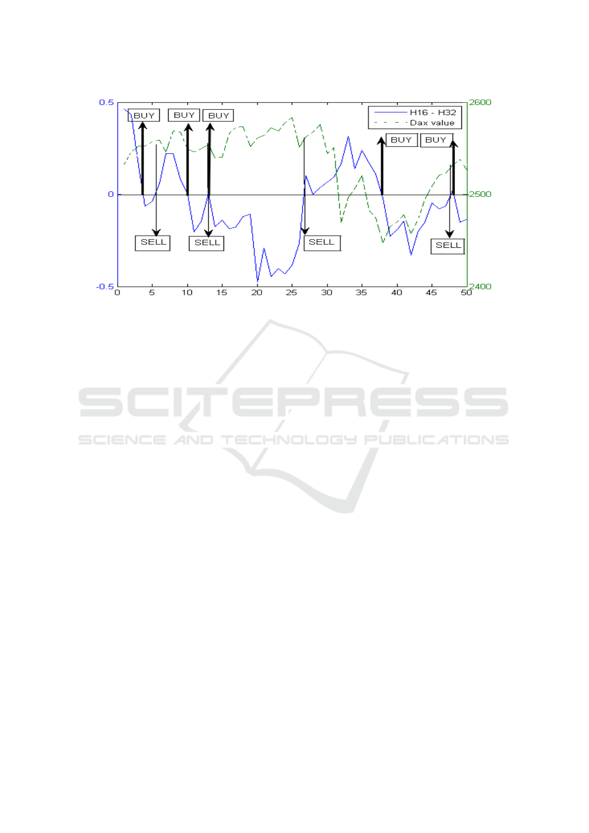
Figure 1: The non-linear MH indicator used for DAX.

produce about three to four time better results than

Buy & Hold strategy in our experiments.

5.1 Hypothesis Testing

Since the differences between proﬁts from the usage

of MACD and MH were ﬂuctuating, we used paired

t-test statistics to test our hypothesis that MH brings

more proﬁt than MACD. We used the time series of

proﬁts generated by MH and the corresponding time

series of proﬁts generated by MACD for all stocks of

DAX and for all stocks of NASDAQ as described in

Section 5. We stated the following two hypotheses:

: µ

= µ

MACD

and

: µ

> µ

MACD

The function used in MatLab was:

alpha = 0.01

test = t.test(macd, y=mh,

alternative=’less’,

paired=TRUE,

conf.level=1-alpha)

The t.test procedure answered for DAX:

t = -6.9046, df = 27, p-value = 1.014e-07

alternative hypothesis:

true difference in means is less than 0

99 percent confidence interval:

-Inf -102.9352

sample estimates:

mean of the differences:

-160.3643

The t.test procedure answered for NASDAQ (data

omitted here):

t = -8.8001, df = 87, p-value = 5.764e-14

alternative hypothesis:

true difference in means is less than 0

99 percent confidence interval:

-Inf -86.42111

sample estimates:

mean of the differences:

-118.2739

So, we reject the theory H

with possible error α =

1% for both data collection (DAX and NASDAQ).

The winning theory is H

, i.e., MH has a greater in-

come rate than MACD.

Similarly, we tested the hypothesis that the using

of MH indicator brings more proﬁt than the using of

Buy & Hold strategy.

5.2 Practical Aspects

However, it must be said that this proﬁt is purely the-

oretical.

First, there is the problem of stationarity explained

in detail in Section 3.3, i.e., the patterns that brought

proﬁt in the past can bring loss in the future, because

the stationarity of market time series is not guaran-

teed, and it is very probably that it is an oversimpliﬁ-

cation.

Second, we have shown that the using of the MH

indicator generated more proﬁt than the using of the

MACD or Buy & Hold strategy, but it can also mean

that the using of both indicators generates a loss, even

though MH generates a smaller loss.

Third, there is the problem of transaction fre-

quency and fees. Usually, at least for small investors,

transactions on stock exchange are charged by fees

ICEIS 2018 - 20th International Conference on Enterprise Information Systems

376

and taxes. Unfortunately, the using of the MH indica-

tor generates a large number of transactions.

We simulated a real investment of 2000 into NAS-

DAQ for a start, and we used the fee of 1% for each

transaction (BUY or SELL) because it corresponds

with the reality. After the whole period (i.e.,1996-

2014), we ﬁnished with 7819.8, and we spent 34497.3

on fees. To make a picture clear, using Buy & Hold

on NASDAQ, we would ﬁnish with 16648.1, and we

would pay only 187.7 for fees.

Tax rules are different in different countries, e.g.,

between 15% − 25%, but it is evident that they re-

duce the proﬁt, too. Usually, the tax has to be paid

immediately after the transaction is ﬁnished. So, the

reinvestment of proﬁt is reduced.

However, the transaction fees depend on the stock

exchange provider. Big investors can use the strategy

of scalping that represents many thousands transac-

tions in a day. Such investors are classiﬁed as market

makers, and they are not charged by transactions fees.

The more detailed explanation is out of the scope of

our paper.

6 CONCLUSIONS

The goal of our investigation was to develop and test

a new indicator MH for technical analysis based on

chaos measure represented by Hurst exponent of the

underlying time series of prices.

We found a construction described in Section 4.1,

and we evaluated it in comparison to the strategy us-

ing MACD or Buy & Hold for data described in Sec-

tion 5.

Using hypothesis testing, we proved our hypothe-

sis that the new MH indicator developed in this work,

i.e., our non-linear method described in Section 4.1,

generates more proﬁt compared to the MACD techni-

cal indicator and to the Buy & Hold investment strat-

egy.

On DAX, MH was 4.5 times better than

Buy & Hold and 7.2 times better than MACD. On

NASDAQ, it was 2.9 times better than Buy & Hold

and 16.8 times better than MACD.

In Subsection 5.2, we explained why the indicator

MH cannot be used as a money generating machine.

However, we believe that complex, non-linear sys-

tems with problematic stationarity are an important

research topic. More research has to be done to an-

swer questions about ﬁltering of BUY- and SELL-

signals. In our future research, we will apply meth-

ods of genetic programming to improve it like in our

previous work (Kroha and Friedrich, 2014).

REFERENCES

Brooks, C. and Persand, G. (2003). Volatility forecasting for

risk management. Journal of Forecasting, 22(1):1–22.

Casdagli, M. (1991). Chaos and deterministic versus

stochastic nonlinear modeling. Technical report,

SFI Working Paper: 1991-07-029, www.santafe.edu

(download 02-26-2017).

Falconer, K. (1990). Fractal Geometry: Mathematical

Foundations and Applications. Wiley.

Fama, E. (1970). Efﬁcient capital markets: A review of the-

ory and empirical work. Journal of Finance, 25:383–

417.

Gleick, J. (1987). Chaos: Making a new Science. Viking

Books.

Gneiting, T. and Schlather, M. (2004). Stochastic models

that separate fractal dimension and the hurst effect.

SIAM Rev, 46:269–282.

Gneiting, T., Sevcikova, H., and Percival, D. B. (2012). Es-

timators of fractal dimension: Assessing the rough-

ness of time series and spatial data. Statistical Science,

27:247–277.

Goldstein, D. G. and Taleb, N. N. (2007). We don’t

quite know what we are talking about when we talk

about volatility. Journal of Portfolio Management,

33(4):84–86.

Hausdorff, F. (1919). Dimension und

außeres maß. Math.

Ann, 79:157–179.

Hurst, H. E. (1951). The long-term storage capacity of

reservoirs. Transaction of the American Society of

Civil Engineers, 116.

Kaplan, I. (2003). Estimating the hurst exponent - c++ soft-

ware source. 1:12.

Kri

stoufek, L. (2010). Rescaled range analysis and de-

trended ﬂuctuation analysis: Finite sample properties

and conﬁdence intervals. AUCO Czech Economic Re-

view, 4(3):315–329.

Kroha, P. and Friedrich, M. (2014). Comparison of genetic

algorithms for trading strategies. In Current Trends

in Theory and Practice of Computer Science - SOF-

SEM 2014, Lecture Notes in Computer Science, vol-

ume 8327, pages 383–394. Springer.

Kroha, P. and Lauschke, M. (2012). Fuzzy and fractal tech-

nology in market analysis. In Studies in Computa-

tional Intelligence - IJCCI 2010, volume 399, pages

247–260. Springer.

Lo, A. W. and MacKinlay, A. C. (1999). A Non-Random

Walk Down Wall Street. Princeton University Press.

Lorenz, E. N. (1963). Deterministic non-periodic ﬂow.

Journal of the Atmospheric Sciences, 2(20):130–141.

Mandelbrot, B. (1963). New methods in statistical eco-

nomics. Journal of Political Economy, 71:421–440.

Mandelbrot, B. (1997). Fractals and Scaling in Finance.

Springer.

Mandelbrot, B. and Hudson, R. L. (2004). The Misbehavior

of Markets. Basic Books.

Mitra, S. K. (2012). Is hurst exponent value useful in fore-

casting ﬁnancial time series? Asian Social Science,

8:8.

Hurst Exponent and Trading Signals Derived from Market Time Series

377

Murphy, J. J. (1999). Technical Analysis of the Financial

Markets: A Comprehensive Guide to Trading Methods

and Applications. New York Institute of Finance.

Nava, N., Di Matteo, T., and Aste, T. (2016). The European

Ohysical Journal Special Topics, 225:1997–2016.

Northington, K. (2009). Volatility-Based Technical Analy-

sis. Wiley.

Peters, E. E. (1994). Fractal Market Analysis - Applying

Chaos Theory to Investment and Economics. Wiley.

Peters, E. E. (1996). Chaos and Order in the Capital Mar-

kets. Wiley, second edition.

Qian, B. and Rasheed, K. (2004). Hurst exponent and ﬁnan-

cial market predictability. In IASTED conference on

Financial Engineering and Applications FEA 2004,

pages 203–209.

Resta, M. (2012). Hurst exponent and its applications in

time-series analysis. Recent Patents on Computer Sci-

ence, 5(3):211–219.

Selvaratnam, S. and Kirley, M. (2006). Predicting stock

market time series using evolutionary artiﬁcial neural

networks with hurst exponent input windows. In Sat-

tar, A. and Kang, B., editors, Advances in Artiﬁcial

Intelligence. AI 2006. Lecture Notes in Computer Sci-

ence, volume 4304, pages 617–626. Springer.

Shleifer, A. (2000). Inefﬁcient Markets – An Introduction to

Behavioral Finance. Oxford University Press.

Skoula, M. (2017). Evaluation of Data from The View-

point of Chaos Theory. Submitted Master Thesis -

FIT CVUT, Praha.

Taleb, N. N. (2007). The Black Swan: The Impact of the

Highly Improbable. Random House.

Vantuch, T. (2014). Impact of hurst exponent on indica-

tor based trading strategies. In Zelinka, I. et al., edi-

tors, : Nostradamus 2014: Prediction, Modeling and

Analysis of Complex Systems, Advances in Intelligent

Systems and Computing 289. Springer.

Weron, R. (2011). Dfa: Matlab function to compute the

hurst exponent using detrended ﬂuctuation analysis

(dfa).

ICEIS 2018 - 20th International Conference on Enterprise Information Systems

378