
Numerical Simulation of Steady State Heat Distribution in Polymer
Concrete Heating with Aggregate Silica Sand and Shellfish
Lukman Hakim
1
and Fauzi
1
1
Department of Physics, Faculty of Mathematics and Natural Sciences, University of Sumatera Utara, USU Campus, Jalan
Bioteknologi No. 1 Medan, 20155, Indonesia
Keywords: Heat Transfer, Polymer Concrete, Simulation Numeric.
Abstract: Environmentally friendly polymer concrete by utilizing waste has been widely developed, one of which is
shellfish waste as filler and silica sand as aggregate. This study was to determine the numerical simulation of
heat distribution during the heating of polymer concrete with steady state with finite difference method of
concrete model polymer and to know thermal conduction characteristics micro . Variation in composition
made of silica sand , seashells (1: 1) or (50 gr: 50gr. Variations in the composition of epoxy resin 25% of the
total weight of sand and shells . The results of this simulation show that the maximum temperature of 80
0
C
is the maximum limit temperature in row one (1) column 2 to 7, row 7 column 2 to 7, and column 7. While
the temperature value of each node is 55 .0987
0
C is on elements (nodes) of five (5) and twenty-five (25).
While most small temperature values are at the nodes of eleven (11) with a value of 3.8333
0
C. heating time
is needed for 360 seconds. From the graph shows that the largest increase in the amount of temperature at
1800 seconds, while the time that shows steady state at 2160 seconds with a fixed value at 80
0
C
1 INTRODUCTION
Computational physics is one of the most important
groups of sciences because it can examine the form of
modeling of complex and complex equations solved
by a numerical approach (Lukman Hakim, 2014).
The finite element method is one of the numerical
methods used to solve equations Partial differential in
engineering science and mathematics problems such
as heat transfer, namely physical dividing complex
problems into elements to make it easier to get
solutions. Solution of each the element is then
combined so that it becomes a problem for the whole
problem (Vimala Rachmawati.,2015).
the research that will be discussed is heat transfer
by solving equations Numerical is the research that
describes the heat transfer elements that are presented
to capture thermal reactions in polymer concrete
which are numerically solved by the finite element
method. The construct equation is criticized into a
series of two-dimensional layers that are related to
finite difference calculations and use the function of
the form of quadrilateral elements (Vimala
Rachmawati.,2015).
Heating a material is the process of transferring
heat from a heat source in the form of a zinc plate
which is useful to find out how fast the heat is moving
and how much heat is occurring in each second. The
heat transfer process is the science of predicting
energy transfer that occurs due to temperature
differences between objects or materials. Steady
conduction heat transfer (steady state) is a conduction
process where the heat value (heat) is equal to time
(Halaudin, 2006).
Concrete is a construction material based on
cement adhesives and aggregates in the form of sand
and gravel (Calvelri, L, Miraglia, N, Papia, M. 2003).
One of the most influential material for polymer
building materials concrete the aggregate of silica
sand and seashell which is expected after testing this
thermal conductivity is having high heat conductivity,
high strength, resistance to corrosion and chemicals
(Shinta Marito, 2009).
Heat transfer in polymer concrete is conduction,
from high-temperature objects to low-temperature
objects that have conductivity properties. the thermal
productivity of a material is the size the ability of
materials to conduct heat (thermal).
Mathematically, the equation of heat distribution
by conduction is formulated:
(1)
Hakim, L. and Fauzi, .
Numerical Simulation of Steady State Heat Distribution in Polymer Concrete Heating with Aggregate Silica Sand and Shellfish.
DOI: 10.5220/0010103910911094
In Proceedings of the International Conference of Science, Technology, Engineering, Environmental and Ramification Researches (ICOSTEERR 2018) - Research in Industry 4.0, pages
1091-1094
ISBN: 978-989-758-449-7
Copyright
c
2020 by SCITEPRESS – Science and Technology Publications, Lda. All rights reserved
1091
Where density, heat type, and
thermal conductivity of the material, respectively, are
the temperature T , and q is the internal nas which is
produced on the material rod.
Equation (1) is solved numerically into equation
(2)
(2)
In equation two (2) is used by the element method
to get a discrete model consisting of a set of piecewise
continuous functions. Each piecewise function is
defined for a sub domain called finite element up to
(Wendy Destyanto, 2007). This concept applies to
problem two. So that equation (2) becomes equation
(3)
(3)
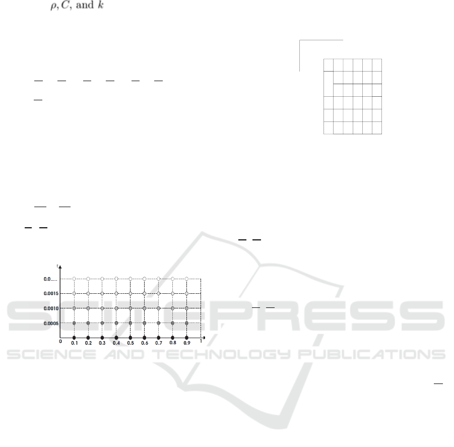
T
Figure1: Mesh-points position. Direction T shows the
position of the points calculated by forward difference,
while t direction shows an increase in time.
2 RESEARCH METHODS
2.1 Modelling
The boundary conditions used in this study are a
polymer concrete sample that is modelled as an area
in the conduction heat flow layer as shown in (1)
below. At the upper and lower limits of the two-
dimensional thermal function network elements,
starting the row matrix (i) and column (j) will be
given a heat source (Q) when heating the polymer
concrete as much as the heat input we want. Then the
thermal will propagate to each row and column
matrix increment, from the row (i = 1) and column (j
= 1) to the end of the row matrix and the column we
want to stop. Dimensional 2 concrete model will be
criticized into a field that has 36 elements and 25 nets.
1
3
4 5
6
7
8
910
11
12
13
14
15
1617
18
1920
21
22
23 24
25
X
Y
2
T=80°C
T=80°C
T=80°C
T=0°C
Figure 2: A model for distributing heat to elements of
polymer concrete.
From equation (3) is converted to discrete or
numeric form, then equation (3) will be equation (4)
(4)
If the width of the grid used is homogeneous and
the same in the direction of x and y, then equation (4)
becomes the equation (5)
(5)
The method used in solving the heat distribution
equation on the material from the Poisson equation
(equation 5) in two dimensions is to use a literature
study or library research approach. The steps in this
study are as follows:
2.1.1 Transform the Poisson equation
along with the condition of the limit
k e Cartesian coordinates
2.1.2 Discretizing the Poisson system on cartesian
coordinates using a network of thermal functions and
boundary conditions.
2.1.3 Substitute the input values of material
conductivity ( k ) and mass density of polymer
concrete ( ρ ) , heat type beto n polymer (Cv) and
source heat (Q) into the Poisson equation in the form
of equations of thermal function networks that have
been obtained.
2.1.4 Calculate the value of the distribution of
Heat T
i, j
in the network of thermal functions.
2.1.5 Perform simulations, draw graphics, and
analyze errors [7].
ICOSTEERR 2018 - International Conference of Science, Technology, Engineering, Environmental and Ramification Researches
1092
3 RESULTS
After doing the stages of the research method, the
following results are obtained:
3.1 The Value of Heat Distribution in
the Polymer Concrete Model in the
Form of a 2-Dimensional Matrix
Measuring 7 Rows and 7 Columns
(7 X 7).
From the data taken from the research of Shinta
Marito, 2019, the results are used as program inputs
with the help of the Matlab program , namely:
3.1.1 The mass of the polymer concrete type ρ =
2716 gram / cm3 in the addition of 80%
seashell powder and 20% epoxy resin,
3.1.2 The heat coefficient of type cv = 90 kcal /
gr
0
C
3.1.3 Heat conductivity K = 0.3 kcal / m
0
C
3.1.4 The initial temperature (T
0
) = 0
0
C
3.1.5 The temperature limit in row 1, row 7 in
column 7 (T
1
) = 80
0
C
Heat distribution results are obtained
3.1.6 Steady state time data ( dt ) = 360 seconds
3.1.7 The ratio parameter value without
dimensions ( rx ) = 0.0442
3.1.8 Temperature distribution value (T) =
0 80.000 80.000 80.000 80.000 80.000 80.00
0 27.646 34.332 36.899 41.821 55.098 80.00
0 8.336 11.732 14.439 21.813 42.100 80.00
0 3.833 5.893 8.486 16.496 38.658 80.00
0 8.336 11.732 14.43 21.813 42.100 80.00
0 27.646 34.332 36.899 41.821 55.098 80.00
0 80.000 80.000 80.000 80.000 80.000 80.00
From the results of the study it was found that the
temperature value of the largest 80
0
C is the
maximum limit temperature in row one (1) column 2
to 7, row 7 column 2 to 7 , and column 7. While the
temperature value of each node is 55 .0987
0
C is
located on elements (nodes) of five (5) and twenty-
five (25). While the smallest temperature value is at
eleven nodes (11) with a value of 3.8333
0
C. This is
due to the number of elements and the number of time
intervals affecting the heat distribution value of each
node. The greater the number of nodes and the longer
the time, the higher the level of accuracy of the heat
distribution value.
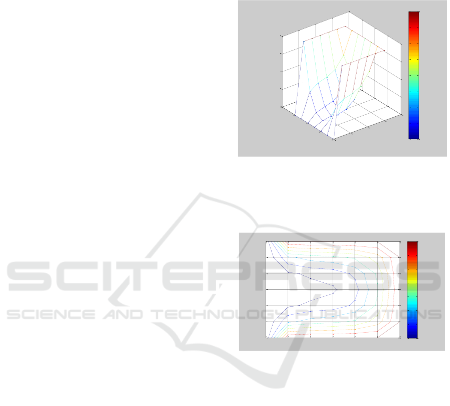
3.2 Heating Results of 2-Dimensional
Polymer Concrete Model
Figure 3: Visualizing heating of polymer concrete 3 (D).
3.3 The Results of Heat Distribution of
2-Dimensional Polymer Concrete
Figure 4: Visualization of heat distribution in 2 D polymer
concrete models.
In the contour chart shows the temperature
distribution varies. In the element area x = 0.1 the area
of heat distribution is wider than in the other elements
this is caused by the initial input value (To) = 0
0
C
and the amount of discretization is small. the more
discretization elements are used then the finer the
resulting contour. This can observed from the
difference in contours in the seven contour lines.
0
0.2
0.4
0.6
0.8
0
0.2
0.4
0.6
0.8
0
20
40
60
80
elements (nodes) on the x axis
the model of heat distribution of polymer concrete in 3 D
Elements (nodes) on the y axis
Temperature
0
10
20
30
40
50
60
70
80
Elements (nodes) on the x axis
Elements (nodes) on the y axiz
Contour of heat distribution at each polymer concrete node
0 0.1 0.2 0.3 0.4 0.5 0.6
0
0.1
0.2
0.3
0.4
0.5
10
20
30
40
50
60
70
80
Numerical Simulation of Steady State Heat Distribution in Polymer Concrete Heating with Aggregate Silica Sand and Shellfish
1093
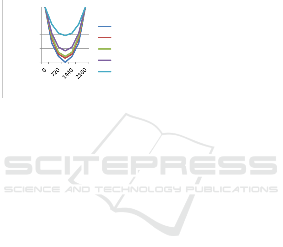
3.4 Analysis of Heating Time to
Increase the Temperature of
Polymer Concrete
Figure 5: Heat distribution of the heating time of polymer
concrete.
From the results of quantitative data that the time
interval (dt) of increasing the number of two-
dimensional elements x and y is 360 second / 0.1
means that each increase in the number of elements,
then the heating time is required by 360 seconds.
From the figure, shows that the largest increase in
range temperature at 1800 seconds, while the time
that shows steady state at 2160 seconds with a fixed
value at 80
0
C this is due to the value of the time of
burning combustion. If the ring number of elements,
and longer, so heat distribution and a steady state will
be clearer.
4 CONCLUSIONS
From the research conducted, some conclusions can
be discribed
a. The program code that is designed in the
research can work well in accordance with the
initial objectives of the study, namely to make
numerical simulations of heat transfer on
polymer concrete. Polymer concrete that is
modeled in two dimensions and has 25 nets
(nodes), is obtained in an interval of 360 seconds
with an error rate of 0.0442 or 4.42% shows that
the largest temperature 55.0987
0
C is located at
nodes 5 and 25. While the lowest temperature is
at node eleven (11) with a value of 3.8333
0
C.
b. Numerically the results of the temperature
distribution of the polymer concrete layer are
influenced by the number of elements used. The
more elements used then the resulting
temperature distribution will increase accurate
even though the numerical changes are not very
significant. This can be observed from changes
in temperature on the corresponding nodes.
c. The number of elements used also affects the
simulation. The more elements used, the more
contour that is produced will be smoother or the
heat transfer becomes more visible for each node
despite the time needed for the simulation will be
longer.
ACKNOWLEDGEMENTS
In this study, the Authors tahnks to Rector of the
University of Sumatera Utara North Sumatra
University Research Institute (USU) for providing
financial support for research grant Talenta 2018 of
young lecturer.
REFERENCES
Lukman Hakim, 2014, Strong Simulation of Magnetic
Fields Near Permanent Magnets Numerical with two-
dimensional requirements around the vacuum, Thesis,
University of North Sumatra
Vimala Rachmawati.,2015, ITS Journal of SCIENCE AND
ART, vol. 4, No.2: 2337-3520
Halaudin, 2006, Gradient Journal vol. 2 No. 2: 152-155
Calvelri, L, Miraglia, N, Papia, M. 2003. Pumice Concrete
For Structural Wall Panel. Belgium: Katholieke
Universiteit Leuven
Shinta Marito, 2009, Utilization of Shellfish and Epoxy
Resin Against Concrete Polymer Characteristics,
Thesis, Medan. University of Northern Sumatra
Wendy Destyanto, 2007, Numerical Simulation of Natural
Convection Heat Transfer in Laminar Flow Limits with
Different Different Methods, Sebelas Maret University
Magical Widodo, M Setyadji, Journal of Materials and
Nuclear Technology, volume 7, no. 22 of 2011: 74-156.
Batan, Serpong
0
20
40
60
80
Heat (
0
C)
Time (secon)
x=0.2
x=0.2
x=0.3
x=0.4
x=0.5
ICOSTEERR 2018 - International Conference of Science, Technology, Engineering, Environmental and Ramification Researches
1094
