Optimization Quantity of Perishable Products Delivery Considering

Total Cost Producer

Abdillah Arief Nasution

, Indah Rizkya

, Khalida Syahputri

, Rahmi M. Sari

, Ikhsan Siregar

and Ivony

Accounting Departement, Faculty of Economic and Business, Universitas Sumatea Utara, Medan, Indonesia

Industrial Engineering, Faculty of Engineering, Universitas Sumatea Utara, Jl. Almamater, Padang Bulan, Medan,

Indonesia

Keywords: Perishable Products.

Abstract: Perishable products is product with a finite lifetime. Perishable products is an expiry date with a fixed lifetime.

Expired time is a problem must be considered in planning of the finished product concerns the product safety

issue when consuming and handling in food industry has its own uniqueness due to the time limit of product

usage. Therefore, analyzing the number of delivery by considering the total cost producer. The research was

conducted to optimize the number of product deliveries to the consumers with consideration of the total cost

producer and expired product becomes reduced. The results obtained by optimizing the number of delivery

based on consideration of total cost producer shows that the optimal number of delivery is 1,081 units with

the total minimum cost producer of Rp. 39.894.900 / month with delivery frequency of 16 delivery / month

and 0.063 month time interval. The total cost of producer can be minimized by 18.7% of the existing total

cost in producer.

1 INTRODUCTION

Food and beverage industry is one of the important

sectors in Indonesian economy because it is able to

contribute to Gross Domestic Product (GDP). This is

evident through the contribution food and beverage

industry into the largest subsector of 34.42%

followed by the growth of food and beverage industry

in 2017 in Indonesia which is increase by 8.15%

(Nafisah, etc, 2016). The food industry is an industry

with a complex supply chain and generally has a great

risk because it produces products with perishable

characteristics.

Perishability is classified in two things, namely

fixed lifetime and random lifetime. Perishable

products is products with a finite lifetime (Joo, etc,

2003). Perishable goods broadly classified into two

categories based on deterioration and obsolescence

(Nagare and Dutta, 2012). Deterioration refers to

damage, spoilage, vaporization, depletion, decay

degradation and loss of potency such as

pharmaceuticals and chemicals of goods.

Obsolescence is value loss of a product due to the

presence of a new product and a better product (Goyal

and Giri, 2001). Fixed lifetime product (such as

human blood used to transfusion, food expiration

limit, etc) has a tend deterministic storage period,

while the random lifetime scenario assumes that the

shelf life at each unit product is a random variable.

Some perishable products will gradually decline

in product quality from time to time (not

spontaneously), deteriorate, until the product ends

completely (broken / expired / unusable). Examples

of products that are susceptible to deterioration in

quality until they are damaged are food, fruits,

vegetables, meat, medicines and medical products.

Most food stuffs, photographic films and

pharmaceutical products is an expiry date with a fixed

lifetime (Ge and Zhang, 2011). Any units remains

unused by expire date considered outdated, and must

be disposed of. Expired time is a problem must be

considered in planning of the finished product

concerns the product safety issue when consuming

(Indrianti, 2001). Therefore handling in food industry

has its own uniqueness due to the time limits of

product usage.

Perishable products problem widely practiced in

previous studies with different perspectives.

(Puspitasari, 2016) Rosi et.al. did a research on

Nasution, A., Rizkya, I., Syahputri, K., Sari, R., Siregar, I. and Ivony, .

Optimization Quantity of Perishable Products Delivery Consider ing Total Cost Producer.

DOI: 10.5220/0010077302130216

In Proceedings of the International Conference of Science, Technology, Engineering, Environmental and Ramiﬁcation Researches (ICOSTEERR 2018) - Research in Industry 4.0, pages

213-216

ISBN: 978-989-758-449-7

213

hospital in Semarang to get an optimal lot size for the

drugs categorized as a deathstroke-return. Another

study also conducted by Ludmila et.al (Dawidowicz

and Postan, 2016) with the problems of perishable

products subject to deterioration during warehousing.

Analyzation and controlling a perishable product to

maintain size of inventory to minimizing the total

cost. The same study also conducted by Dalfard and

Nosratian (Dalfard and Nosratian, 2014) described a

pricing constrained single-product and inventory-

production model in perishable food with

deterioration rate to maximizing the total profit.

However, studies on perishable inventory issues

has been done before did not consider the total cost

incurred by the producer in optimizing the delivery

and this study aims to optimize the number of

delivery with the consideration of total cost producer

and expired products become reduced.

2 METHODOLOGY

The research was conducted on one of the industries

producing perishable products in the form of cakes

with various types. The object in this study is the total

of expired products produced on SMEs. The research

begins by making observations directly to SMEs to

see the conditions existing in the SMEs. By making

observations, will be obtained problems occurs in

SMEs and will be determined Formulation of the

problem according to the real condition.

Based on the formulation of the problem,

determined the purpose of research as a solution in

analyzing and handling these condition. Next stage,

problem solving using supporting data as an input in

problem solving. The data used in handling the

problem of products number expired and high cost of

returns in the form of the request numbers per

product, product capacity, delivery frequency,

product purchasing price, ordering costs, delivery

costs, storage costs, and expired costs.

Based on these data, calculates the optimal

number of delivery by considering the total cost

producer and the number of expired products to be

reduced. The calculation of the optimal number of

delivery is done by several stages. The first stage is to

calculate the aggregate demand. The aggregate

demand is obtained by determining the conversion

factor first. The conversion factor is determined by

looking at the minimum raw material requirements in

producing at each product.

After obtaining the number of demand in

aggregate units, the next step is to determine the total

delivery. Total delivery can be obtained by

determining the time interval and the size of the

finished pr/duct delivery lot first. The time interval is

obtained from the ratio between the planning cycle

(T) and the delivery frequency (n). The time interval

calculation can be done using the formula (Rau, etc,

2004):

Time Interval (t) =

(1)

And the calculation of lot size in finished product

delivery is done by using formula:

Delivery Lot Size(q

) =

θB

θBt

-1]

(1)

D is a product demand for a month while "θB"

represents the rate of damage to the finished product

to the consumer. Based on these two formulas, we

will get the total delivery at each delivery frequency

by multiplying the delivery time interval which is

obtained by the size of the finished product delivery

lot.

The next step is to calculate the producer’s total

cost. This calculation is done to determine the total

cost expenses due to many expire products and done

immediately. Calculation of total cost of producer is

done by using the formula:

Total Cost Producer = Setup Cost +

Delivery Finished Product Cost + Storage

Finished Product Cost + Expired Cost of

Produce

(1)

Setup cost is the cost expenses when an order is

filed with the formula. Delivery cost is the cost

expenses when the finished product is delivered to the

consumer. Storage costs represent expenses for

maintenance purposes, rental of premises, or

insurance cost on products / raw materials available.

And expired cost is the cost expenses because the

products passed the life already (Limansyah and

Lesmono, 2011). Based on the value at each cost, the

total cost will be obtained for the producer and the

total optimal product delivery determined by

considering the minimum total cost of producer.

3 RESULT AND DISCUSSION

3.1 Aggregate Demand

Calculation of aggregate demand is done by

determining the convection factor first. Based on the

raw materials needed to produce each product, it is

found that brownies products have the minimum

requirement of raw material among other products

ICOSTEERR 2018 - International Conference of Science, Technology, Engineering, Environmental and Ramiﬁcation Researches

214

with the total of flour 0.10 kg / product and brownies

product becomes conversion factor in calculating

aggregate demand. The aggregate demand is

calculated by multiplying the demand for the finished

product for 30 days with the conversion at each

product. The calculation of aggregate demand is

calculated in daily for each product for 30 days.

Based on the calculation, it is found that the number

of demand for finished products in aggregate demand

about 17,099.3 brownies units for 30 days.

3.2 Delivery Lot Size

The calculation of the delivery lot size is obtained by

determining the time interval value and size of the

finished product delivery lot first. Based on the

formula used in calculating the total number of

delivery, it is found that the size of the finished

product delivery lot with the frequency of product

delivery 16 times in 30 days is 1,081 with the total

delivery of the finished prodct optimally about 17,304

units of brownies.

3.3 Total Cost

The total cost calculated in this research is the total

cost of producers. Total cost is obtained based on the

value of other costs required in producing the product

from setup costs, storage costs, delivery costs, and

expired costs for products passed through life. Based

on the value of these costs, it is found that the total

cost for the optimal number of product delivery is Rp.

39.894.900 / month. Recapitulation of total optimal

delivery and total cost producer can be seen in Table

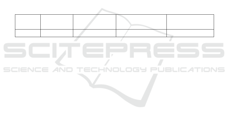
Table 1: Recapitulation of Total Optimal Delivery and Total Cost Producer.

Frequency

Time Interval Delivery Lot Size Total of Optimal

Delivery

Total Cost

16 0,063 month 1.081 unit brownies 17.305 unit brownies Rp. 39.894.900/month

Based on the table above, obtained that the total

minimum cost of the producer is Rp. 39.894.900 /

month with the delivery frequency 16 times of the

delivery / month and the time interval of 0.063

months and lot size of 1,081 units brownies. The

results of this study were carried out with other

studies that have been conducted on the inventory of

perishable products. Determination of the optimal lot

size (Q) on the manufacturer that is capable of filling

the total number of shipments and total producers

(Puspitasari, etc, 2016) (Limansyah and Lesmono,

2011).

The existing condition of producer do daily

delivery to agent with total delivery 30 times in a

month. The producer total cost can be minimized by

18.7% of the existing total cost in producer. The

existing condition delivered product every day, so

cost of delivery increased.

4 CONCLUSIONS

Perishable products is an expiry date with a fixed

lifetime. Expired time is a problem must be

considered in planning of the finished product

concerns the product safety issue when consuming

and handling in food industry has its own uniqueness

due to the time limit of product usage.

By optimizing the number of delivery time based

on the consideration of total cost producers, it is

found that total optimal delivery of 1,081 units with

the total minimum cost of the producer is Rp.

39.894.900/month with delivery frequency of 16

delivery / month and 0.063 month time interval.

ACKNOWLEDGEMENTS

This work has been fully supported by TALENTA

Research Program from Universitas Sumatera Utara

with the number of contract

2590/UN5.1.R/PPM/2018, March 16th, 2018.

Author would like to thank to all of participants who

have a role in conducting of this study.

REFERENCES

L Nafisah, W Sally, and Puryani, 2016. Jurnal Teknik

Industri, 18 (1) 63-72.

Optimization Quantity of Perishable Products Delivery Considering Total Cost Producer

215

K Y Joo, K C Soo, H Hark 2003 Asia Pacific Management

Review, 8 (4) 509-521.

M Nagare, and P Dutta 2012. Proceeding of the

International Multi Conference of Engineers and

Computer Scientists Vol II March 14-16, Hongkong

S K Goyal, B C Giri 2001 European Journal of Operational

Research, 134 (1) 1-16.

Y Ge and J Zhang 2011. Journal of Service Science and

Management, 4 (4) 440- 444.

N Indrianti, M Tjen, and I S Toha 2001. Jurnal Media

Teknik, (2)

R Puspitasari, A Arvianto, D I Rinawati, and P W Laksono

2016 2

International Conference of Industrial,

Mechanical, Electrical, Chemical Engineering

(ICIMECE)

L F Dawidowicz, and M Postan 2016. Scientific Journal of

Logistic, 12 (2) 147-156.

V M Dalfard, N E Nosratian 2014. Neural Computing and

Applications, 24 (3) 735-734.

H Rau, M Y Wee, and H M Wee 2004. International

Journal of System Science, 35 (5) 293-303.

T Limansyah, D Lesmono 2011. Jurnal Teknik Industri, 13

(2) 87-94.

ICOSTEERR 2018 - International Conference of Science, Technology, Engineering, Environmental and Ramiﬁcation Researches

216