ANFIS Synthesis by Clustering for Microgrids EMS Design

Stefano Leonori, Alessio Martino, Antonello Rizzi and Fabio Massimo Frattale Mascioli

Department of Information Engineering, Electronics and Telecommunications,

University of Rome ”La Sapienza”, Via Eudossiana 18, 00184 Rome, Italy

Keywords:

Smart Grids, Microgrids, Energy Management System, ANFIS, Data Clustering, Decision Making System.

Abstract:

Microgrids (MGs) play a crucial role for the development of Smart Grids. They are conceived to intelligently

integrate the generation from Distributed Energy Resources, to improve Demand Response (DR) services, to

reduce pollutant emissions and curtail power losses, assuring the continuity of services to the loads as well. In

this work it is proposed a novel synthesis procedure for modelling an Adaptive Neuro-Fuzzy Inference Sys-

tem (ANFIS) featured by multivariate Gaussian Membership Functions (MFs) and ﬁrst order Takagi-Sugeno

rules. The Fuzzy Rule Base is the core inference engine of an Energy Management System (EMS) for a grid-

connected MG equipped with a photovoltaic power plant, an aggregated load and an Energy Storage System

(ESS). The EMS is designed to operate in real time by deﬁning the ESS energy ﬂow in order to maximize the

revenues generated by the energy trade with the distribution grid. The ANFIS EMS is synthesized through

a data driven approach that relies on a clustering algorithm which deﬁnes the MFs and the rule consequent

hyperplanes. Moreover, three clustering algorithms are investigated. Results show that the adoption of k-

medoids based on Mahalanobis (dis)similarity measure is more efﬁcient with respect to the k-means, although

affected by some variety in clusters composition.

1 INTRODUCTION

A Microgrid (MG) is an electric grid able to in-

telligently manage and control local electric power

systems affected by stochastic and intermittent be-

haviours, such as electric generation from renewable

energy sources, electric vehicles charging and de-

ferrable and shiftable loads. MGs are the best can-

didates for the transition to Smart Grids, since they

allow a bottom-up approach for building and devel-

oping reliable and smart distribution systems, relying

on the concept of territorial granulation. Each MG

is provided of a suitable Energy Management Sys-

tem (EMS) to intelligently manage local power ﬂows

inside MG and with the main grid (Patterson, 2012;

Dragicevic et al., 2014). The MG infrastructure relies

on power converters connecting power systems and

electric loads to the main bus in order to locally route

and manage the MG power ﬂows and the power ex-

changes with the connected grid. To this end, MGs

must be equipped with a communication infrastruc-

ture able to monitor and supervise the state of all the

MG components.

Usually, MGs are supported by Energy Storage Sys-

tems (ESSs) able to guarantee both the quality of ser-

vice and the electric stability, ensuring some energetic

autonomy to the system when it is disconnected to

the grid (

i.e.

islanded mode). The implementation

of a suitable Demand Side Management (DSM) EMS

allows to apply Demand Response (DR) services to

the costumer, which is more appropriate to refer to as

prosumer whether equipped with a power generation

system.

In (Deng et al., 2015) are well summarized all the DR

main services (i.e. valley ﬁlling, load shifting, peak

shaving operations). These services, together with

Vehicle-2-Grid (V2G) operations and the intelligent

use of the ESS, allow to reduce the stress caused by

the MG to the connected distribution grid in order to

get incentives, avoid penalties, reduce both the con-

sumptions and the operational costs, which strictly

depend on the energy price policies adopted by the

distribution grid. Concerning this topic, in (Kirschen,

2003; Amer et al., 2014) are discussed the develop-

ment of new energy policies which will involve the

costumer to assume an active role in the energy mar-

ket by means of the application of DR services.

In this work, a procedure based on computational in-

telligence techniques for the data driven synthesis of

an EMS is proposed. The EMS must deﬁne in real

time the energy ﬂow exchanged with the grid in or-

der to maximize the MG proﬁt by considering a Time

Leonori S., Martino A., Rizzi A. and Frattale Mascioli F.

ANFIS Synthesis by Clustering for Microgrids EMS Design.

DOI: 10.5220/0006514903280337

In Proceedings of the 9th International Joint Conference on Computational Intelligence (IJCCI 2017), pages 328-337

ISBN: 978-989-758-274-5

Of Use (TOU) energy policy. The MG EMS is based

on an Adaptive Neuro-Fuzzy Inference System (AN-

FIS) that is efﬁciently modelled by a clustering algo-

rithm. In addiction, different clustering algorithms

are investigated and compared for the ANFIS mod-

elling, which mainly differ in the (dis)similarity mea-

sure adopted. Moreover,it is also investigated the efﬁ-

cacy of considering the EMS output space by the clus-

tering algorithms (i.e. joint input-output space) rely-

ing on a benchmark solution found through a Mixed-

Integer Linear Programming (MILP) problem formu-

lation.

The remainder of the paper is organized as follows.

In Sec. 2 is introduced the MG problem formulation.

The EMS design and the modelling procedure are

described in Sec. 3, where both the Objective Func-

tion (OF) formulation and the set of clustering algo-

rithms will be introduced. In Sec. 5 are reported the

simulations settings, whereas the achieved results are

in Sec. 6, followed by the conclusions discussed in

Sec. 7.

2 MG PROBLEM FORMULATION

In this paper it is considered a prosumer grid-

connected MG equipped with a DSM EMS. It is in

charge of efﬁciently manage the MG components rep-

resented as aggregated systems grouped in renewable

sources power generators, electric loads and ESSs.

Their energy ﬂows are managed in real time by an

EMS that acts as decision making system. It must ef-

ﬁciently redistribute the prosumer energy balance (i.e

the overall energy produced net of the energy demand

at the given time slot) between the grid and the ESS

by maximizing the proﬁt given by the energy trade

with the main grid.

This work is based on several hypotheses which help

deﬁning the correct level of abstraction to properly

focus the problem under analysis as made in previ-

ous studies (Leonori et al., 2016a; Leonori et al.,

2016b). The power value of the MG components

has been considered constant within each 15 min-

utes time slot. Low level operations such as voltage

and reactive power control are not considered. The

power transmission losses within the MG are consid-

ered negligible. The on-line control module ensures

that the power balance is achieved during the real-

time operation. The EMS has a sample time equal to

the time slot duration which is considerably greater

than the characteristic time of the ESS power con-

trol, therefore the ESS inner loop has been neglected.

The power converters which connect the MG sub-

components to each other, included the one allow-

ing the MG-grid connection, are neglected in terms

of power losses and characteristic time of control.

The MG aggregated energy generation, aggregated

load request, energy exchanged with the ESS and en-

ergy exchanged with the grid during the n

time slot

are denoted with E

, E

and E

, respectively. In

ﬁgure 1 it is represented a schematic diagram of the

MG where the power lines are drawn in black and the

signal wires in red. In Figure is also represented the

Battery Management System (BMS). It monitors the

ESS and estimates its State Of Charge (SoC) which is

used as an input of the EMS.

n−1

SoC

n−1

sell

n−1

, C

buy

n−1

Figure 1: MG architecture. Signal wires in red, power lines

in black.

By assuming that the prosumer energy production E

has the priority to meet the prosumer energy demand

, the prosumer energy balance E

can be deﬁned

= E

+ E

, n = 1, 2, ... (1)

in each time slot.

Moreover, in this work it is assumed that the prosumer

energy balance E

is a known quantity read in real

time by an electric meter. In each time slot, E

must

be exchanged with the main grid and the ESS by ful-

ﬁlling the following energy balance relation

+ E

= 0, n = 1, 2, ... (2)

The energy E

is assumed positive or negative when

the ESS is discharged or recharged, respectively. Sim-

ilarly, the energy E

is considered positive (negative)

when the network is selling (buying) energy to the

MG. Considering a TOU price policy, it is possible to

formulate the proﬁt P generated by the energy trade

with the main grid in a time period composed by N

slot

time slots as

P =

slot

∑

n=1

where P

(

·C

buy

if E

> 0

·C

sell

if E

≤ 0

(3)

where C

buy

and C

sell

deﬁne the energy prices in pur-

chase and sale during the n

time slot. According

with (Leonori et al., 2017), it is assumed that dur-

ing the n

time slot the MG cannot exchange with

the grid an amount of energy greater than the current

energy balance E

. In other words, in case of over-

production (over-demand) (i.e. E

> 0 (E

< 0))

the ESS can be only charged (discharged).

In this work the EMS is assumed to be able to efﬁ-

ciently estimate in real time the energy E

and E

be exchanged during the n

time slot with the con-

nected grid and the ESS, respectively (see ﬁgure 1).

The EMS is supposed to be fed by the input vector u

constituted by 4 variables, namely, the current energy

balance E

n−1

, the current energy prices in sale and

purchase, C

sell

n−1

and C

buy

n−1

and the SoC value Soc

n−1

It should be noted that whereas E

n−1

, C

sell

n−1

and C

buy

n−1

are instantaneous quantities read by proper meters,

SoC

n−1

is a status variable depending on the previous

ESS history. Before entering the EMS, the E

, C

sell

buy

inputs, must be normalized in the range [0, 1],

whilst the SoC belongs to [0, 1] by its own deﬁnition.

In the following, the normalized input vector will be

referred to as

3 PROBLEM STATEMENT AND

MODELLING APPROACH

The use of computational intelligence techniques and,

especially, Fuzzy Logic and Fuzzy Inference Systems

(FISs), is often mentioned in literature for solving

the EMS real time decision making system design.

In such cases, the inferential process (i.e. the rule

based system) can be realized relying on expert op-

erator(s) with the support of heuristics, such as Ge-

netic Algorithms (GAs). Moreover, Mamdani FIS

types based on grid partitioning, are the most com-

monly used due to their simplicity and effectiveness.

For example in (Arcos-Aviles et al., 2016) is proposed

a GA-FIS model in order to minimize the power peaks

and the ﬂuctuations of the energy exchange with the

connected-grid, while keeping the battery SoC within

certain security limits; in (Leonori et al., 2016b) a rule

base system designed by an expert operator has been

optimized by a GA in order to maximize the proﬁt

generated by the energy trade with the main grid as-

suming a TOU energy price. In these works, the ap-

plication of heuristics, speciﬁcally GAs, has been mo-

tivated by the fact that the synthesis problem has been

casted as an unsupervised one.

In this paper it is proposed an EMS synthesis proce-

dure in a supervised fashion. To this end, the EMS

model has been synthesized through an ANFIS sup-

ported by clustering. The proposed paradigm is well

introduced in (Panella et al., 2001).

The supervised problem formulation needs to rely on

a ground-truth output values solution, namely the de-

sired output E

. In this regard, a benchmark solution

has been evaluated through a MILP formulation.

The adoption of such synthesis procedure with a su-

pervised formulation allows to avoid both expert op-

erator(s) and heuristics, at least for a preliminary

study. Converselyto Mamdani FIS type, the proposed

model, based on Takagi-Sugeno formulation, is not

sensitive to the MF resolution or, in other words, the

spatial granularity. Moreover, it does not need an a-

priori analysis of the GA complexity and efﬁciency,

that is strictly related to the FIS number of parame-

ters to be tuned.

3.1 ANFIS EMS Structure

ANFIS models are one of the most popular type of

fuzzy artiﬁcial neural networks. They are composed

by 7 layers. As well described in (Jang, 1993), AN-

FISs implement FISs by means of a suitable set of

ﬁrst order Takagi-Sugeno rules. The generic j

rule

has the form:

if x

is Φ

( j)

and ... x

is Φ

( j)

then y =

∑

i=1

( j)

+ θ

( j)

(4)

where x = [x

, ..., x

] is a generic crisp input vector.

Each x

is evaluated by the respective rule antecedent

term set, deﬁned by the Fuzzy Set MF Φ

. The second

term y is the output associated to the j

rule. It is es-

timated through the calculation of the associated rule

consequent hyperplane, deﬁned by the coefﬁcients θ

In this work it has been decided to deﬁne every rule

antecedent by a unique MF. Therefore, the ANFIS

MFs are modelled by means of multivariate Gaus-

sian functions which assure the coverage of the entire

fuzzy domain regardless of the number of employed

MFs. The generic MF Φ(

u), where the input vector ¯u

has been introduced in Sec. 2, is deﬁned as follows:

Φ(

u) = e

−

(

u−µ

µ)·C

−1

·(

−µ

)

(5)

where µ

µ and C are the mean vector value and the co-

variance matrix of the multivariate Gaussian function,

respectively. The consequent fuzzy rule is modelled

as in (4). The rule consequent outputs E

, the energy

exchanged with the grid, that is evaluated by means

of a suitable hyperplane deﬁned as follows:

= θ

+ θ

sell

+ θ

buy

+ θ

SoC (6)

The overall output of the ANFIS is computed by

adopting a Winner Takes All strategy. All rule

weights are ﬁxed to unitary values.

3.2 Benchmark Solutions and Objective

Function Formulation

Algorithms based on MILP, along with Dynamic Pro-

gramming and Linear Programming, namely methods

able to ﬁnd an optimal solution through a determinis-

tic (or sub-optimal since MILP is supported by heuris-

tics) approach, are suitable for the determination of a

benchmark solution (Sundstrom and Guzzella, 2009)

useful to validate and support the EMS modelling.

In this case, it supports the EMS modelling by casting

the problem from unsupervised to supervised learn-

ing. Speciﬁcally, the ANFIS model is trained on a

given dataset together with its respective benchmark

solution found through a MILP formulation of the

problem, by re-adapting the approach proposed in

(Palma-Behnke et al., 2013). By deﬁning P

upper

and

lower

as the MILP optimal solution obtained with and

without the ESS, respectively, the OF in ((3)) can be

rewritten as:

P =

upper

− P

upper

− P

lower

(7)

Such proﬁt normalization allows to estimate how

much the EMS performances are close to the opti-

mal solution considering a given dataset. The respec-

tive upper benchmark solution ESS SoC proﬁle and

proﬁle are named SOC

opt

and E

opt

, respectively.

These are used for the EMS synthesis procedure.

3.3 ANFIS Synthesis by Clustering

In literature, several techniques to train an AN-

FIS architecture have been analyzed. For example,

backpropagation-based and clustering-based training

have been proposed in (Jang, 1993) and (Rizzi et al.,

1999), respectively. In this work, the latter technique

is adopted. It exploits a clustering algorithm in or-

der to build the ANFIS architecture, in particular the

MFs’ shape and the rule based system.

Speciﬁcally, three different clustering algorithms are

introduced and successively compared for the EMS

synthesis problem. By starting from the widely-

known k-means algorithm (MacQueen, 1967; Lloyd,

1982), the others are mainly re-adaptations and/or ex-

tensions of it (still, well-known in literature) in or-

der to explore and implement different (dis)similarity

measures. Moreover, it is discussed how to take ad-

vantage of the output space (i.e. the E

opt

benchmark

solution) in case of clustering in the so-called joint

input-output space, as explained in (Panella et al.,

2001).

3.3.1 k-means

k-means is an hard partitional clustering algorithm

which, given a dataset S = { x

, x

, ..., x

}, re-

turns k non-overlapping groups (clusters), i.e. S =

, ..., S

}, such that S

∩S

0 if i 6= j and ∪

i=1

S, such that objects in the same cluster are more simi-

lar to each other than to those in other clusters. In or-

der to ﬁnd such clusters, k-means aims at minimizing

the following objective function, namely the Within-

Cluster Sum-of-Squares (WCCS):

WCSS =

∑

i=1

∑

x∈S

kx− r(i)k

(8)

where kx − r(i)k

is the squared Euclidean distance

between pattern x and the i

cluster representa-

tive r(i), usually known as centroid, deﬁned as the

component-wise mean amongst patterns in cluster

. Minimizing (8) is, however, an NP-hard problem

(Aloise et al., 2009) and what is commonly known as

k-means is actually an heuristic which, as such, does

not guarantee to ﬁnd an optimal solution. k-means

is based on the Voronoi iteration or, equivalently, an

Expectation-Maximization algorithm which works as

follows:

i Select k initial centroids according to some

heuristics (e.g. randomly);

ii Assignment (Expectation) Step: assign each pat-

tern to nearest cluster (closest centroid);

iii Update (Maximization) Step: update clusters’

centroids;

iv Loop ii–iii until a given stopping criterion is met

(e.g. maximum number of iterations is reached or

centroids’ update is below a given threshold).

3.3.2 k-medians

A commonly used variant of the k-means algorithm

consists in changing the (dis)similarity measure from

squared Euclidean distance to 1-norm (also known as

Manhattan, TaxiCab or CityBlock distance), leading

to the so-called k-medians problem (Bradley et al.,

1997).

The 1-norm (dis)similarity measure implies to con-

sider the Assignment Step and the OF (9) with no

squares involved, but considering the absolute value

only. Therefore, the k-medians OF shall be referred

to as, more generally, the Within-Clusters Sum-of-

Distances (WCSD):

WCSD =

∑

i=1

∑

x∈S

kx− r(i)k

(9)

k-medians still works by the Expectation-

Maximization steps introduced in Sec. 3.3.1.

However, in this case the cluster’s representative is

the median, evaluated by taking the component-wise

median rather than the mean amongst patterns in

clusters. Due to the minimization of the 1-norm

rather than squared 2-norm, k-medians is more robust

to noise and outliers with respect to k-means; indeed,

the median is not (so-much) skewed in presence of

(few) very low or very high values.

3.3.3 k-medoids

In k-medoids (Kaufman and Rousseeuw, 1987) the

cluster’s representative (known as medoid or Min-

SOD

) is the cluster datapoint which minimizes the

sum of distances within the cluster itself. Conversely

to k-means and k-median, in k-medoids clusters’ rep-

resentatives are actual members of the dataset at hand

by deﬁnition. In this work, the k-medoids problem

has been solved by means of the implementation pro-

posed in (Park and Jun, 2009), which is based to the

same Voronoi iterations at the basis of k-means and k-

medians. k-medoids, due to the representatives’ deﬁ-

nition, can ideally deal with any (dis)similarity mea-

sures. Therefore, its objective function can generally

be deﬁned as

WCSD =

∑

i=1

∑

x∈S

D(x− r(i)) (10)

where D(·, ·) is the (dis)similarity measure. In this

paper, the adopted (dis)similarity measure for k-

medoids is the Mahalanobis distance (Mahalanobis,

1936), deﬁned as following:

d(x, r(i)) =

(x− r(i))

· C

−1

· (x− r(i)) (11)

where C

is the covariance matrix for the i

cluster

and r(i) is its representative (i.e. the medoid).

Since the k-medoids algorithm minimizes the sum of

pairwise distances rather than the sum of squares, it

is more robust to noise and outliers with respect to

k-means.

3.3.4 ANFIS Synthesis by Joint Input-output

Space Clustering

Albeit clustering is an unsupervised problem by

deﬁnition, the dataset at hand consists in la-

belled patterns; thus, it has the form S =

{(x

, y

), (x

, y

), ..., (x

, y

)} where x

∈ R

and

∈ R, for i = 1, ..., N

, which we refer to as input and

output space(s), respectively. Since in this work the

Minimum Sum Of Distances

clustering problem in the joint input-output space will

be considered, the cluster’s representative(s) must be

re-deﬁned. Indeed, if one has to work in the in-

put space (i.e. with unlabelled patterns), the clus-

ters’ representatives as deﬁned in Secs. 3.3.1–3.3.3

sufﬁce. Conversely, as concerns joint input-output

spaces, each cluster will be described by:

• its original representative r (either mean, median

or medoid – depending on the algorithm at hand)

• its covariance matrix C

• a set of N

+ 1 coefﬁcients θ

The former two quantities will be used in order to

build the ANFIS MF according to (5), whereas the

latter will be used in order to deﬁne the hyperplane

which locally approximates the input-output mapping

according to (6). Speciﬁcally, it can be evaluated us-

ing the Least Mean Squares (LMSs) estimator:





−1

(12)

where X

is the set of input patterns lying in the i

cluster and Y

is the set of corresponding output val-

ues (ground-truth). It is worth noticing that patterns

in X

will be augmented by appending a heading 1

such that their dimension is N

+ 1: in this manner

∈ R

, as it also considers the hyperplane’s in-

tercept (cf. (6)).

In order to fully consider both the input and out-

put spaces, the (dis)similarity measure has been

readapted, regardless of the speciﬁc adopted cluster-

ing algorithm. The pattern-to-cluster (dis)similarity

measure is deﬁned as a convex linear combination

between the point-to-representative distance (input

space) and the approximation error given by the in-

terpolating hyperplane (output space):

d(x, hr, C, θ

θi) = ε · d(x, r) + (1− ε)



y− θ

· x



(13)

where d(·, ·) is one of the given (dis)similarity mea-

sures (either squared Euclidean, Manhattan or Maha-

lanobis), the triad hr, C, θ

θi, as introduced, deﬁnes the

fuzzy rule and, ﬁnally, ε ∈ [0, 1] is a trade-off param-

eter which tunes the linear convex combination. It is

worth noticing that if ε = 1 the rightmost term in (13)

will not be considered, thus collapsing into a standard

clustering problem.

The rationale behind (13) is that the algorithm aims

at minimizing the approximation error due to the hy-

perplane (rightmost term) and, at the same time, at

discovering well-formed

clusters in the input space

(leftmost term).

either compact or homogeneous, depending on the

(dis)similarity measure and, by extension, on the clustering

algorithm objective function

4 EMS MODELLING

PROCEDURE

In this section is explained in details how the ANFIS

EMS is efﬁciently modelled through the exploitation

of a clustering algorithm. The ANFIS optimization

process is explained from a generic point of view,

valid for each clustering algorithm proposed in the

previous section, including their variants (i.e. along

with the output space). The clustering algorithm re-

lies on a given dataset composed by E

, C

buy

and

sell

time series.

The whole dataset has been partitioned in TrS,

VlS and TsS (i.e. Training Set, Validation Set and

Test Set, respectively). These are used to train the

ANFISs, to select the best for a given number of MFs

and to measure the performances of the optimum one,

respectively. The dataset partition among TsS, TrS

and VlS is made on a daily base, namely all time slots

associated with the same day will belong to a sin-

gle set. More precisely, the whole dataset is ﬁrstly

divided in two subsets having the same cardinality.

The ﬁrst subset constitutes the TsS whereas the sec-

ond one is partitioned in 5 different ways in order to

constitute 5 different TrS and VlS pairs.

Algorithm 1 EMS Training Procedure

1: procedure EMS DESIGN

2: TsS and hTrSs,VlSsi pairs partitioning

3: for j = 1 to 5 do ⊲ for each TrS

4: {E

opt

, SoC

opt

}

:= MILP(TrS

)

5: ⊲ evaluation of the optimal solution

6: Γ

:= {TrS

, SoC

opt

, E

opt

}

7: ⊲ Clustering input dataset

8: end for

10: for k = 2 to 25 do ⊲ for each value of k

11: for j = 1 to 5 do ⊲ for each TrS

12: {µ

, C

, θ

} := clustering(k, Γ

)

13: Φ

:= {µ

, C

} ⊲ MF evaluation

14: ANFIS

:= {Φ

, θ

}

15: simulation of ANFIS

on VlS

→

16: end for

17: selection of ANFIS

best

according with

18: simulation of ANFIS

best

on the TsS → P

19: end for

20: end procedure

The clustering procedure exploits the generic TrS

dataset, namely the TrS of the j

TrS-VlS pair, to-

gether with the corresponding optimum proﬁles of

(SoC

opt

)

and (E

opt

)

found through the MILP opti-

mization. For the sake of ease, the dataset read by

the clustering algorithm is deﬁned by Γ

. It is clear

that if the only EMS input space is considered, (E

opt

)

will not take part as a feature for clustering and will

be only used for the estimation of the hyperplanes co-

efﬁcients deﬁned by θ

, once they are deﬁned (see

(12)). Conversely, if the clustering procedure is ap-

plied on the joint input-output space, the coefﬁcients

are updated after each Voronoi iteration together

with the clusters. The optimization process is ran for

a number of clusters k ranging from k = 2 to k = 25

on the j

dataset Γ

For each k, the clustering procedure is repeated for

each Γ

(i.e. 5 times), returning the respective k

representative vectors, covariance matrices and hy-

perplanes coefﬁcients. These are used to model the

ANFIS multivariate Gaussian MFs Φ

(i.e. rule an-

tecedent set) and the Sugeno hyperplanes (i.e. rule

consequent set) represented by the θ

coefﬁcient

sets, respectively, according to (5) and (6), as intro-

duced in Sec.3.3.4. The previously described pro-

cedure results in 24 × 5 different ANFIS synthesis.

More precisely, for each k value there exist 5 dif-

ferent ANFIS corresponding to the 5 different TrSs.

Each generated ANFIS is then simulated on its re-

spective VlS and its performance is evaluated accord-

ing to (7). For each value of k, the best ANFIS among

the 5 TrS-VlS pairs, named ANFIS

best

, is selected

whereas the remaining 4 are discarded. Finally, for

each ANFIS

best

the MG EMS is simulated on the TsS

in order to evaluate the generalization capability. The

overall procedure of the EMS ANFIS design and op-

timization is illustrated in Algorithm 1.

5 SIMULATION SETTINGS

In this work it has been considered a MG composed

by the following energy systems: a PV generator of

19 kW, an aggregated load with a peak power around

8 kW, and ESS with an energy capacity of 24 kWh.

For the ESS modelling it has been taken into consid-

eration the Toshiba ESS SCiB module having a rated

voltage of 300 V, a current rate of 8 C-Rate and a ca-

pacity of about 80 Ah.

The dataset used in this work has been provided by

AReti S.p.A., the electricity distribution company in

Rome. The energy prices are the same used in pre-

vious works, (Leonori et al., 2016a; Leonori et al.,

2016b).

The considered dataset covers an overall period of 20

days, sampled with a 15 minutes frequency. The over-

all dataset is shown in ﬁgure 2, together with the en-

ergy prices both in sale (positive) and purchase (neg-

ative).

0 200 400 600 800 1000 1200 1400 1600 1800

-2

-1

Generation Demand

sell

buy

kWh, SoC, MU

time slot

Figure 2: MG power production and demand of the overall

dataset and TOU energy prices.

The even days are assigned to the TsS, whereas the

odd days are partitioned with a random selection be-

tween the TrS and VlS in order to form 5 different

TrS-VlS partitions (see Sec. 4). It has been chosen

to assign the 70% of the odd days to the TrS and the

remaining 30% to the VlS.

The ANFIS optimization process is executed for each

clustering algorithm introduced in Sec. 3.3 and by

varying the ε values, namely the local approximation

error inﬂuence, as follows:

• k-means for ε equal to 1, 0.75, 0.5 and 0.25.

• k-medians for ε equal to 1, 0.75, 0.5 and 0.25.

• k-medoids for ε equal to 1, 0.75, 0.5 and 0.25.

The clustering algorithms have been set with a max-

imum number of iterations equal to 50 and every ex-

ecution of the algorithm (i.e. number of replicates) is

repeated 20 times with a new, random, initial repre-

sentatives selection.

The solution chosen by the clustering algorithm af-

ter each run is the one which minimizes its respective

objective function (see Sec. 3.3), namely the WCCS

deﬁned in (8) for k-means, (9) for k-medians and (10)

for k-medoids.

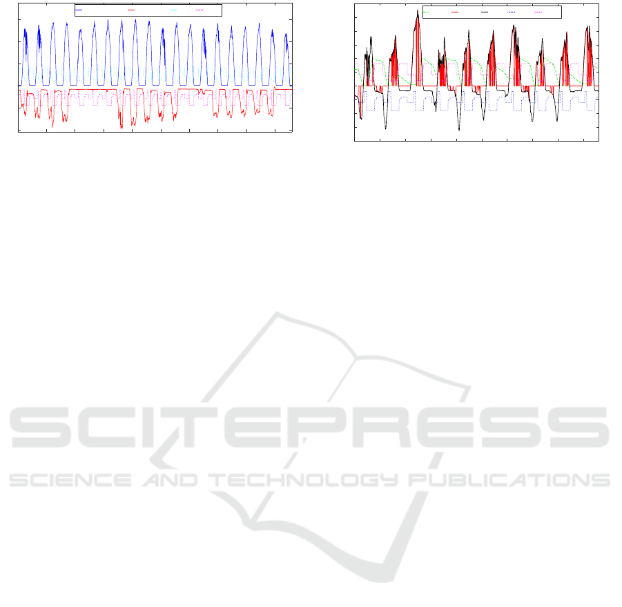
6 RESULTS

The simulation results have been studied by comput-

ing the OF

P deﬁned in (7) on the TsS, whose optimal

solution is shown in ﬁgure 3.

The results on the TsS given by the procedure de-

scribed in Algorithm 1 are shown in ﬁgure 4, as a

function of k, by reporting the respective value of

P for each ANFIS

best

generated. These are grouped

by the different ε coefﬁcient values, which range be-

tween 1 and 0.25 as deﬁned in Sec. 5. It is possi-

ble to observe that k-medoids in most cases presents

the best results, being its OF curves (in green) lower

with respect to the other two competitors (k-means

in red and k-medians in blue). Moreover, for lower

0 100 200 300 400 500 600 700 800 900

-2

-1.5

-1

-0.5

0.5

1.5

2.5

SOC

−E

buy

sell

kWh, SoC, MU

time slot

Figure 3: MG optimum solution energy ﬂows, ESS SoC and

energy prices computed on the TsS by MILP approach.

values of ε, especially for ε = 0.25 (i.e. when the

approximation error due to hyperplane prevails (see

(13)), the k-medoids results appear to be more sta-

ble as k increases with respect to the other two algo-

rithms (see ﬁgure 4-d). k-means and k-medians show

a smoother behaviour of

P, especially for ε = 1 (ﬁg-

ure 4-a), meaning that these are more stable when

considering the input space only. In all cases their

proﬁt results are around 80% of the optimum solu-

tion.

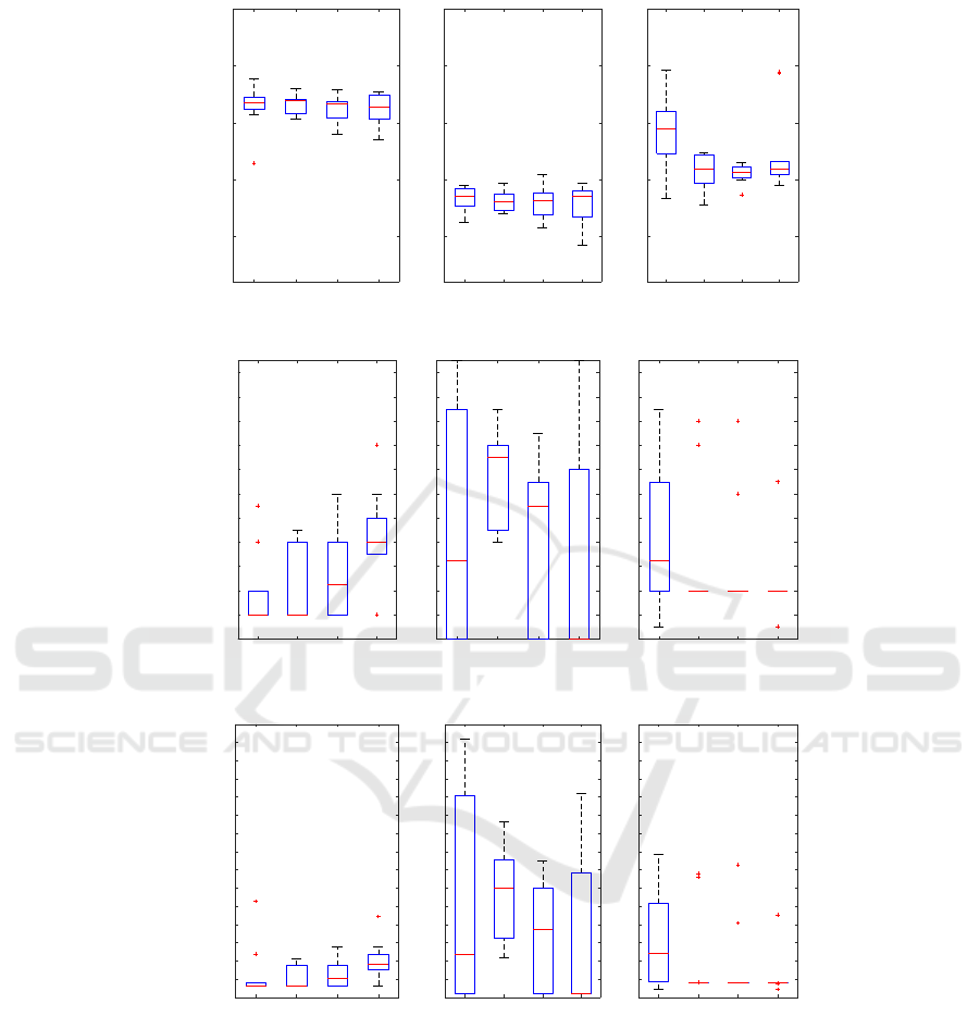
In order to focus on the results reliability and sen-

sitivity, the carried out tests have been repeated 10

times. In this study, for the sake of clarity, it has

been decided to select only ANFIS

best

associated with

the best OF result on the TsS. The selected solu-

tions are displayed through a boxplot representation

in ﬁgure 5 after being grouped by ε coefﬁcient and

clustering algorithm. Speciﬁcally, in ﬁgure 5-a are

reported the ANFIS

best

selected solution OF (

P) val-

ues; in ﬁgure 5-b their respective number of clusters

and, ﬁnally, in ﬁgure 5-c are reported the Davies-

Bouldin Index (DBI) values (Davies and Bouldin,

1979), which measures both intra-clusters compact-

ness and inter-clusters separation.

As shown in ﬁgure 5-a, best results are conﬁrmed

to be prevalently given by k-medoids. These are

followed by the k-medians. On the other hand, k-

medoids solutions present high level of variability

both on the value of k and the DBI, as pointed by

higher extension of the boxes (see ﬁgure 5-b and

c). Nevertheless, for ε = 0.5 the boxplots show a

lower variance for

P, k and DBI. In k-means and k-

medians solutions, considering the joint input-output

space term seems to be scarcely signiﬁcant. Only

for k-means the joint input-output space term in OF

yields a relevant improvement in terms of reduction

of the DBI and the number of clusters. More into

details, as far as k-medoids is concerned, by look-

ing at the DBI it is possible to see that the clustering

2 5 10 15 20 25

0.2

0.4

0.6

k-means k-medians k-medoids

2 5 10 15 20 25

0.2

0.4

0.6

2 5 10 15 20 25

0.2

0.4

0.6

2 5 10 15 20 25

0.2

0.4

0.6

ε = 1

ε = 0.75

ε = 0.5

ε = 0.25

Figure 4: ANFIS

best

normalized proﬁt values evaluated on TsS as a function of k. Solutions are grouped according to ε.

problem is hard to solve

, whereas the k-means and

k-medians lead to better solutions. However, in terms

of OF (see (7)) k-medoids overperforms the other two

competitors. This is mainly due to the Mahalanobis

distance which, by considering up to the second-order

statistics (i.e. the covariance matrix), is aware of the

clusters’ shapes as well. Indeed, by using the Ma-

halanobis distance k-medoids effectively updates the

covariance matrix at each iteration, conversely to the

other two clustering-based ANFIS synthesis proce-

dures, where the covariance matrix is evaluated once,

at the end of the clustering procedure.

7 CONCLUSION

In this work it has been investigated a procedure for

the synthesis of a MG EMS based on computational

intelligence techniques. It performs a cluster analysis

in order to ﬁnd automatically the number and the lo-

cation on the input space of the rules composing an

ANFIS, as the core inference engine of the EMS.

The ANFIS synthesis is casted as a supervised ma-

chine learning problem, where patterns are input-

output pairs, taking as ground-truth output values the

ones coming from the benchmark solution obtained

by a MILP procedure.

In particular, three considered clustering algorithms

have been compared, which differ for their respective

(dis)similarity measures and the way clusters’ repre-

sentatives are evaluated. Besides, a clustering proce-

Recall: the lower DBI, the better the partition. Indeed,

a low DBI means low intra-variance (high compactness)

and high inter-variance (high separation).

dure in the joint input-output space has been inves-

tigated, evaluating its effectiveness when the weight-

ing coefﬁcient in the OF changes. Results show that

adopting the Mahalanobis distance on the joint input-

output space leads to proﬁts way superior than k-

means. This improvements, however, are paid with

higher values of both the average number of clusters

(i.e. model complexity) and its variance (i.e. algo-

rithm robustness).

On the other hand, the adoption of the k-medians

seems a good compromise in terms of both robust-

ness and effectiveness of OF performance and par-

titions quality in terms of DBI. Starting from these

ﬁndings, further experiments can be done. First, it is

possible to adopt a hierarchical clustering algorithm

in order to better deal with larger datasets, improving

both speed and accuracy in clusters discovery. More-

over, a genetic algorithm can be applied to tune the

ANFIS parameters (De Santis et al., 2017) (e.g. rule

weights and MF shape) once it is synthesised by the

clustering algorithm.

REFERENCES

Aloise, D., Deshpande, A., Hansen, P., and Popat, P. (2009).

Np-hardness of euclidean sum-of-squares clustering.

Machine learning, 75(2):245–248.

Amer, M., Naaman, A., M’Sirdi, N. K., and El-Zonkoly,

A. M. (2014). Smart home energy management sys-

tems survey. In International Conference on Renew-

able Energies for Developing Countries 2014, pages

167–173.

Arcos-Aviles, D., Pascual, J., Marroyo, L., Sanchis, P.,

and Guinjoan, F. (2016). Fuzzy logic-based en-

ergy management system design for residential grid-

connected microgrids. IEEE Transactions on Smart

Grid, PP(99):1–1.

Bradley, P. S., Mangasarian, O. L., and Street, W. N. (1997).

Clustering via concave minimization. In Advances

in neural information processing systems, pages 368–

374.

Davies, D. L. and Bouldin, D. W. (1979). A cluster separa-

tion measure. IEEE Transactions on Pattern Analysis

and Machine Intelligence, PAMI-1(2):224–227.

De Santis, E., Rizzi, A., and Sadeghian, A. (2017). Hier-

archical genetic optimization of a fuzzy logic system

for energy ﬂows management in microgrids. Applied

Soft Computing, 60:135 – 149.

Deng, R., Yang, Z., Chow, M. Y., and Chen, J. (2015). A

survey on demand response in smart grids: Mathemat-

ical models and approaches. IEEE Transactions on

Industrial Informatics, 11(3):570–582.

Dragicevic, T., Vasquez, J. C., Guerrero, J. M., and Skrlec,

D. (2014). Advanced lvdc electrical power architec-

tures and microgrids: A step toward a new generation

of power distribution networks. IEEE Electriﬁcation

Magazine, 2(1):54–65.

Jang, J.-S. (1993). Anﬁs: adaptive-network-based fuzzy in-

ference system. IEEE transactions on systems, man,

and cybernetics, 23(3):665–685.

Kaufman, L. and Rousseeuw, P. (1987). Clustering by

means of medoids. Statistical data analysis based on

the L1-norm and related methods.

Kirschen, D. S. (2003). Demand-side view of electric-

ity markets. IEEE Transactions on Power Systems,

18(2):520–527.

Leonori, S., De Santis, E., Rizzi, A., and Frattale Mascioli,

F. M. (2016a). Multi objective optimization of a fuzzy

logic controller for energy management in microgrids.

In 2016 IEEE Congress on Evolutionary Computation

(CEC), pages 319–326.

Leonori, S., De Santis, E., Rizzi, A., and Frattale Masci-

oli, F. M. (2016b). Optimization of a microgrid en-

ergy management system based on a fuzzy logic con-

troller. In IECON 2016 - 42nd Annual Conference of

the IEEE Industrial Electronics Society, pages 6615–

6620.

Leonori, S., Paschero, M., Rizzi, A., and Frattale Masci-

oli, F. M. (2017). An optimized microgrid energy

management system based on ﬁs-mo-ga paradigm. In

2017 IEEE International Conference on Fuzzy Sys-

tems (FUZZ-IEEE), pages 1–6.

Lloyd, S. (1982). Least squares quantization in pcm. IEEE

transactions on information theory, 28(2):129–137.

MacQueen, J. (1967). Some methods for classiﬁcation and

analysis of multivariate observations. In Proceed-

ings of the ﬁfth Berkeley symposium on mathematical

statistics and probability, volume 1, pages 281–297.

Oakland, CA, USA.

Mahalanobis, P. C. (1936). On the generalised distance in

statistics. Proceedings of the National Institute of Sci-

ences of India, 1936, pages 49–55.

Palma-Behnke, R., Benavides, C., Lanas, F., Severino, B.,

Reyes, L., Llanos, J., and Sez, D. (2013). A micro-

grid energy management system based on the rolling

horizon strategy. IEEE Transactions on Smart Grid,

4(2):996–1006.

Panella, M., Rizzi, A., Frattale Mascioli, F. M., and Mar-

tinelli, G. (2001). Anﬁs synthesis by hyperplane clus-

tering. In Proceedings Joint 9th IFSA World Congress

and 20th NAFIPS International Conference (Cat. No.

01TH8569), volume 1, pages 340–345 vol.1.

Park, H.-S. and Jun, C.-H. (2009). A simple and fast algo-

rithm for k-medoids clustering. Expert systems with

applications, 36(2):3336–3341.

Patterson, B. T. (2012). Dc, come home: Dc microgrids and

the birth of the ”enernet”. IEEE Power and Energy

Magazine, 10(6):60–69.

Rizzi, A., Frattale Mascioli, F. M., and Martinelli, G.

(1999). Automatic training of anﬁs networks. In Fuzzy

Systems Conference Proceedings, 1999. FUZZ-IEEE

’99. 1999 IEEE International, volume 3, pages 1655–

1660 vol.3.

Sundstrom, O. and Guzzella, L. (2009). A generic dynamic

programming matlab function. In 2009 IEEE Control

Applications, (CCA) Intelligent Control, (ISIC), pages

1625–1630.

0.25 0.5 0.75 1

0.15

0.175

0.2

0.225

0.25

0.25 0.5 0.75 1

0.15

0.175

0.2

0.225

0.25

0.25 0.5 0.75 1

0.15

0.175

0.2

0.225

0.25

k-means k-medoids k-medians

0.25 0.5 0.75 1

k-means k-medoids k-medians

0.25 0.5 0.75 1

0.5

1.5

2.5

3.5

4.5

5.5

6.5

7.5

0.25 0.5 0.75 1

0.5

1.5

2.5

3.5

4.5

5.5

6.5

7.5

0.25 0.5 0.75 1

0.5

1.5

2.5

3.5

4.5

5.5

6.5

7.5

DBI

k-means k-medoids k-medians

Figure 5: Simulation results on TsS considering the best solution of each run illustrated through a box-plot representation. Top

and bottom box sides correspond to ﬁrst and third quantiles, respectively, whereas the red dash corresponds to the median. Top

and bottom whiskers extremities correspond to the maximum and minimum points not considered as outliers, respectively.

These latter are marked with a red + symbol. In (a) are shown the OF values; in (b) the number of MFs; in (c) the DBI

associated to the clustering solution which models each ANFIS.