Unsupervised Segmentation of Hyper-spectral Images via Diffusion Bases
Alon Schclar
1
and Amir Averbuch
2
1
School of Computer Science, The Academic College of Tel-Aviv Yaffo, POB 8401, Tel Aviv 61083, Israel
2
School of Computer Science, Tel Aviv University, POB 39040, Tel Aviv 69978, Israel
Keywords:
Segmentation, Diffusion Bases, Dimensionality Reduction, Hyper-spectral Sensing.
Abstract:
In the field of hyper-spectral sensing, sensors capture images at hundreds and even thousands of wavelengths.
These hyper-spectral images, which are composed of hyper-pixels, offer extensive intensity information which
can be utilized to obtain segmentation results which are superior to those that are obtained using RGB images.
However, straightforward application of segmentation is impractical due to the large number of wavelength
images, noisy wavelengths and inter-wavelength correlations. Accordingly, in order to efficiently segment the
image, each pixel needs to be represented by a small number of features which capture the structure of the
image. In this paper we propose the diffusion bases dimensionality reduction algorithm (Schclar and Averbuch,
2015) to derive the features which are needed for the segmentation. We also propose a simple algorithm for the
segmentation of the dimensionality reduced image. We demonstrate the proposed framework when applied
to hyper-spectral microscopic images and hyper-spectral images obtained from an airborne hyper-spectral
camera.
1 INTRODUCTION
Image segmentation is the process of partitioning an
image into disjoint subsets of pixels in which pixels
belong to the same subset are more similar than pix-
els that belong to different subsets. Each subsets is
referred to as a segment.
A regular CCD camera provides very limited
spectral information as it is equipped with sensors that
only capture details that are visible to the naked eye.
However, a hyper-spectral camera is equipped with
multiple sensors - each sensor is sensitive to a partic-
ular range of the light spectrum including spectrum
ranges that are not visible to the naked eye - namely,
infra-red and ultra-violet. Its output contains the re-
flectance values of a scene at all the wavelengths of
the sensors. Hyper-spectral cameras can be hand held
(Zheludeva et al., 2015) or they can be mounted on
airplanes (e.g. (Tarabalka et al., 2010)) or micro-
scopes (Cassidy et al., 2004).
A hyper-spectral image is composed of a set of
images - one for each wavelength. We refer to a set
of wavelength values at a coordinate (x, y) as a hyper-
pixel. Each hyper-pixel can be represented by a vector
in R
n
where n is the number of wavelengths. This
data can be used to achieve inferences that can not be
derived from a limited number of wavelengths which
are obtained by regular cameras.
Commonly, the number of wavelengths is much
higher than the actual degrees of freedom of the data.
Unfortunately, this phenomenon is usually unavoid-
able due to the inability (lack of knowledge which
sensor values are more important for the task at hand)
to produce a special sensor for each application. Con-
sider for example a task that separates red objects
from green objects using an off-the-shelf digital cam-
era. In this case, the camera will produce, in addition
to the red and green channels, a blue channel, which
is unnecessary for this task.
Naturally, effective utilization of the wealth of
wavelengths can yield segmentation results that are
better than those obtained by merely using RGB data,
for example, by incorporating infra-red and ultra-
violet wavelengths. One can simply apply classi-
cal image processing techniques to each wavelength
image individually. However, this will not utilize
inter-wavelength connections, which are inherent in
spectral signatures. Furthermore, the high number of
wavelengths renders the application of segmentation
algorithms to the entire hyper-spectral image useless
due to the curse of dimensionality. Thus, the entire
hyper-spectral cube needs to be processed in order to
analyze the physical nature of the scene. Naturally,
this has to be done efficiently due to the large volume
of the data.
Typical hyper-spectral images contain a high de-
Schclar A. and Averbuch A.
Unsupervised Segmentation of Hyper-spectral Images via Diffusion Bases.
DOI: 10.5220/0006503503050312
In Proceedings of the 9th International Joint Conference on Computational Intelligence (IJCCI 2017), pages 305-312
ISBN: 978-989-758-274-5
Copyright
c
 2017 by SCITEPRESS – Science and Technology Publications, Lda. All rights reserved

gree of correlation between many of the wavelengths
which renders many of them redundant. Moreover,
certain wavelengths contain noise as a result of poor
lighting conditions and the physical condition of the
camera at the time the images were captured. Ac-
cordingly, the noise and the redundant data need to be
removed while maintaining the information which is
vital for the segmentation. This information should be
represented as concisely as possible i.e. each hyper-
pixel should be represented using a small number of
attributes. This will alleviate the curse of dimension-
ality and allow the efficient application of segmen-
tation algorithms to the concisely represented hyper-
spectral image. To achieve this, dimensionality reduc-
tion needs to be applied to the hyper-spectral image.
In this paper we propose to reduce the dimen-
sionality of the hyper-spectral image by using the re-
cently introduced diffusion bases (DB) dimension-
ality reduction algorithm (Schclar and Averbuch,
2015). The DB algorithm efficiently captures non-
linear inter-wavelength correlations and produces a
low-dimensional representation in which the amount
of noise is drastically reduced. We also propose a fast
and simple histogram-based segmentation algorithm
which will be applied to the low-dimensional repre-
sentation.
We use a simple and efficient histogram-based
method for automatic segmentation of hyper-spectral
volumes in which the DB algorithm plays a key role.
The proposed method clusters hyper-pixels in the
reduced-dimensional space. We refer to this method
as the Wavelength-wise Global (WWG) segmentation
algorithm.
This paper is organized as follows: in section 2
we present a survey of related work on segmenta-
tion of hyper-spectral images. The diffusion bases
scheme (Schclar and Averbuch, 2015) is described in
section 3. In section 4 we introduce the two phase
Wavelength-wise Global (WWG) segmentation algo-
rithm. Section 5 contains experimental results from
the application of the algorithm to several hyper-
spectral images. Concluding remarks are given in sec-
tion 6.
2 RELATED WORKS
Segmentation methods for hyper-spectral images can
be divided into two categories - supervised and unsu-
pervised. Supervised methods segment the image us-
ing either a-priori spectral information of the sought
after segments or information regarding the shape of
the segments. Some methods use both types of in-
formation. Unsupervised segmentation techniques do
not utilize any a-priori information. The method pro-
posed in this paper falls into the latter category.
The method in (Ye et al., 2010) uses both a-priori
spectral information and shape information of the seg-
ments. Specifically, they use the model which is pro-
posed in (Chan et al., 2006) which is a covexifica-
tion of the two-phase version of the Mumford-Shah
model. The model uses variational methods to find a
smooth minimal length curve that divides the image
into two regions that are as close as possible to being
homogeneous. The a-priori spectral and shape infor-
mation is incorporated in the variational model and its
optimization.
In (Li et al., ) a variational model for simul-
taneous segmentation and denoising/deblurring of a
hyper-spectral image which models the image as a
set of three-dimensional tensors. The spectral signa-
tures of the sought after materials is known a-priori
and is incorporated in the model. The segmentation
is obtained via a statistical moving average method
which uses the spatial variation of spectral correla-
tion. Specifically, a coarse-grained spectral correla-
tion function is computed over a small moving 2D
spatial cell of fixed shape and size. This function pro-
duces sharp variations as the averaging cell crosses a
boundary between two materials.
In (Li et al., 2010) a supervised Bayesian seg-
mentation approach is proposed. The method makes
use of both spectral and spatial information. The
two-phase algorithm first implements a learning
step, which uses the multinomial logistic regres-
sion via variable splitting and augmented (LORSAL)
(Bioucas-Dias and Figueiredo, 2009) algorithm to in-
fer the class distributions. A segmentation step fol-
lows which infers the labels from a posterior distribu-
tion built on the learned class distributions. A max-
imum a-posterior (MAP) segmentation is computed
via a min-cut based integer optimization algorithm.
The algorithm also implement an active learning tech-
nique based on the mutual information (MI) between
the MLR regressors and the class labels in order to
reduce the size of the training set.
In (Tarabalka et al., 2010) an extension to the the
watershed (Vincent and Soille, 1991) segmentation
algorithm is proposed. Specifically, the algorithm is
used to to define information about spatial structures
and uses one-band gradient functions. The segmen-
tation maps are incorporated into a spectral–spatial
classification scheme based on a pixel-wise Support
Vector Machine classifier.

3 THE DIFFUSION BASES
DIMENSIONALITY
ALGORITHM
The Diffusion bases (DB) dimensionality reduction
algorithm (Schclar and Averbuch, 2015) reduces the
dimensionality of a dataset by utilizing the inter-
coordinate variability of the original data (in this
sense it is dual to the Diffusion Maps algorithm (Coif-
man and Lafon, 2006; Schclar, 2008; Schclar et al.,
2010)). It first constructs the graph Laplacian using
the image wavebands as the datapoints. It then uses
the Laplacian eigenvectors as an orthonormal system
and projects the hyper-pixels on it. The eigenvectors
are sorted in descending order according to their mag-
nitude and only the eigenvectors that correspond to
the highest eigenvalues are used. These eigenvectors
capture the non-linear coordinate-wise variability of
the original data. Although bearing some similarity
to PCA, this process yields better results than PCA
due to: (a) its ability to capture non-linear manifolds
within the data by local exploration of each coordi-
nate; (b) its robustness to noise. Furthermore, this
process is more general than PCA and it produces
similar results to PCA when the weight function w
ε
is linear e.g. the inner product.
Let Γ =
{
x
i
}
m
i=1
, x
i
∈ R
n
, be the original dataset of
hyper-pixels and let x
i
( j) denote the j-th coordinate
(the reflectance value of the j-th band) of x
i
, 1 ≤ j ≤
n. We define the vector x
0
j
, (x
1
( j), . . . , x
m
( j)) to be
the j-th coordinate of all the points in Γ i.e. the image
corresponding to the j-th band.. We construct the set
Γ
0
=

x
0
j

n
j=1
. (1)
Let w
ε
(x
i
, x
j
), be a weight function which measures
the pairwise similarity between the points in Γ
0
. A
Markov transition matrix P is constructed by normal-
izing the sum of each row in the matrix w
ε
to be 1:
p

x
0
i
, x
0
j

=
w
ε

x
0
i
, x
0
j

d (x
0
i
)
where d (x
0
i
) =
∑
n
j=1
w
ε

x
0
i
, x
0
j

. Next, eigen-
decomposition of p

x
0
i
, x
0
j

is performed
p

x
0
i
, x
0
j

≡
n
∑
k=1
λ
k
ν
k

x
0
i

µ
k

x
0
j

where the left and the right eigenvectors of P are
given by
{
µ
k
}
and
{
ν
k
}
, respectively, and
{
λ
k
}
are the
eigenvalues of P in descending order of magnitude.
We use the eigenvalue decay property of the eigen-
decomposition to extract only the first η(δ) eigenvec-
tors B ,
{
ν
k
}
k=1,...,η(δ)
which contain the non-linear
directions with the highest variability of the coordi-
nates of the original dataset Γ. We project the orig-
inal data Γ onto the basis B. Let Γ
B
be the set of
these projections: Γ
B
=
{
g
i
}
m
i=1
, g
i
∈ R
η(δ)
, where
g
i
=

x
i
· ν
1
, . . . , x
i
· ν
η(δ)

, i = 1, . . . , m and · denotes
the inner product operator. Γ
B
is the reduced dimen-
sion representation of Γ and it contains the coordi-
nates of the original points in the orthonormal system
whose axes are given by B.
4 THE WAVELENGTH-WISE
GLOBAL (WWG)
SEGMENTATION ALGORITHM
We introduce a simple and efficient two-phase ap-
proach for the segmentation of hyper-spectral im-
ages. The first phase reduces the dimensionality of
the data using the DB algorithm and the second stage
applies a histogram-based method to cluster the low-
dimensional data.
We model a hyper-spectral image as a three di-
mensional cube where the first two coordinates cor-
respond to the position (x, y) and the third coordinate
corresponds to the wavelength λ
k
. Let
I =
n
p
λ
k
i j
o
i, j=1,...,m;k=1,...,n
∈ R
m×m×n
(2)
be a hyper-spectral image cube, where the size of the
image is m × m and n is the number of wavelengths.
For notation simplicity, we assume that the images
are square. It is important to note that almost always
n  m
2
.
I can be viewed in two ways:
1. Wavelength-wise: I =

I
λ
l

is a collection of n
images of size m × m where
I
λ
l
,

p
λ
l
i j

∈ R
m×m
, 1 ≤ l ≤ n (3)
is the image that corresponds to wavelength λ
l
.
2. Point-wise: I =
n
−→
I
i j
o
m
i, j=1
is a m × m collection
of n-dimensional vectors where
−→
I
i j
,

p
λ
1
i j
, . . . , p
λ
n
i j

∈ R
n
, 1 ≤ i, j ≤ m (4)
is the hyper-pixel at position (i, j).
The proposed WWG algorithm assumes the
wavelength-wise setting of a hyper-spectral image.
Thus, we regard each image as a m
2
- dimensional
vector. Formally, let
˜
I ,

π
i,λ
l

i=1,...,m
2
;l=1,...,n
∈ R
m
2
×n
(5)

be a 2-D matrix corresponding to I where
π
i+( j−1)·m,λ
k
, p
λ
k
i j
, 1 ≤ k ≤ n , 1 ≤ i, j ≤ m,
(p
λ
k
i j
is defined in Eq. 2) and let
˜
I
λ
k
,



π
1,λ
k
.
.
.
π
m
2
,λ
k



∈ R
m
2
, 1 ≤ k ≤ n (6)
be a column vector that corresponds to I
λ
k
(see Eq.
3).
4.1 Phase 1: Reduction of
Dimensionality via DB
Different sensors can produce values at different
scales. Thus, in order to have a uniform scale for all
the sensors, each column vector
˜
I
λ
k
, 1 ≤ k ≤ n, is nor-
malized to be in the range [0,1].
We form the set of vectors Γ =

˜
I
λ
1
, . . . ,
˜
I
λ
n

from
the columns of
e
I and we apply the DB Algorithm to
Γ. We denote the dimension-reduced representation
of Γ by Γ
B
.
4.2 Phase 2: Histogram-based
Segmentation
We introduce a histogram-based segmentation algo-
rithm that extracts objects from Γ using Γ
B
. For no-
tation convenience, we denote η (δ) − 1 by η here-
inafter. We denote by G the cube representation of
the set Γ
B
in accordance with Eq. 2:
G ,

g
k
i j

i, j=1,...,m;k=1,...,η
, G ∈ R
m×m×η
.
We assume a wavelength-wise setting for G. Let
e
G
be a 2-D matrix in the setting defined in Eq. 5
that corresponds to G. Thus, G
l
,

g
l
i j

i, j=1,...,m
∈
R
m×m
, 1 ≤ l ≤ η corresponds to a column in
e
G and
−→
g
i j
,

g
1
i j
, . . . , g
η
i j

∈ R
η
, 1 ≤ i, j ≤ m corresponds
to a row in
e
G. The coordinates of
−→
g
i j
will be referred
to hereinafter as colors.
The segmentation is achieved by clustering hyper-
pixels with similar colors. This is based on the as-
sumption that similar objects in the image will have a
similar set of color vectors in Γ
B
. These colors con-
tain the correlations between the original hyper-pixels
and the global inter-wavelength changes of the im-
age. Thus, homogeneous regions in the image have
similar correlations with the changes i.e. close colors
where closeness between colors is measured by the
Euclidean distance.
The segmentation-by-colors algorithm consists of
the following steps:
1. Normalization of the Input Image Cube G:
First, we normalize each wavelength of the image
cube to be in [0,1]. Let G
k
be the k-th (k is the
color index) color layer of the image cube G. We
denote by
b
G
k
=

b
g
k
i j

i, j=1,...,m
the normalization
of G
k
and define it to be
b
g
k
i j
,
g
k
i j
− min

G
k

max
{
G
k
}
− min
{
G
k
}
, 1 ≤ k ≤ η. (7)
2. Uniform Quantization of the Normalized Input
Image Cube
b
G:
Let l ∈ N be a given number of quantization lev-
els. We uniformly quantize every value in G
k
to
be one of l possible values. The quantized matrix
is given by Q:
Q ,

q
k
i j

i, j=1,...,m;k=1,...,η
, q
k
i j
∈
{
1, . . . , l
}
(8)
where q
k
i j
=
j
l ·
b
g
k
i j
k
. We denote the quantized
color vector at coordinate (i, j) by
−→
c
i j
,

q
1
i j
, . . . , q
η
i j

∈ R
η
, 1 ≤ i, j ≤ m. (9)
3. Construction of the Frequency color His-
togram:
We construct the frequency function
f :
{
1, . . . , l
}
η
→ N where for every
κ ∈
{
1, . . . , l
}
η
, f (κ) is the number of quan-
tized color vectors
−→
c
i j
, 1 ≤ i, j ≤ η, that are
equal to κ.
4. Finding Peaks in the Histogram:
Local maxima points (called peaks) of the fre-
quency function f are detected. We assume that
each peak corresponds to a different object in
the image cube G. Here we use the classical
notion of segmentation - separating object from
the background. Indeed, the highest peak cor-
responds to the largest homogeneous area which
in most cases is the background. The histogram
may have many peaks. Therefore, we perform
an iterative procedure to find the θ highest peaks
where the number θ of sought after peaks is given
as a parameter to the algorithm. This param-
eter corresponds to the number of objects we
seek. The algorithm is also given an integer
parameter ξ, which specifies the l
1
cube radius
around a peak. We define the ξ-neighborhood of
a coordinate (x
1
, · ·· , x
η
) to be N
ξ
(x
1
, · ·· , x
η
) =

{(y
1
, · ·· , y
η
)
|
max
k
{|
y
k
− x
k
|}
≤ ξ }. The coordi-
nates outside the neighborhood N
ξ
are the can-
didates for the locations of new peaks. An it-
erative procedure is used in order to find all the
peaks. The peaks are labeled 1, . . . , θ. The out-
put of the algorithm is a set of vectors Ψ =

−→
ρ
i

i=1,...,θ
,
−→
ρ
i
=

ρ
1
i
, . . . , ρ
η
i

∈ N
η
that con-
tains the highest peaks. A summary of this step
is given in algorithm 1.
5. Finding the Nearest Peak to each color:
Once the highest peaks are found, each quantized
color vector is associated with a single peak. The
underlying assumption is that the quantized color
vectors, which are associated with the same peak,
belong to the same object in the color image cube
I. Each quantized color is associated with the
peak that is the closest to it with respect to the Eu-
clidean distance. Each quantized color is labeled
by the number of its associated peak. We denote
by
γ:
−→
c
i j
7→ d ∈
{
1, . . . , θ
}
this mapping function, where
γ(
−→
c
i j
) , arg min
1≤k≤θ
n


ρ
k
−
−→
c
i j


l
η
o
.
6. Construction of the Output Image:
The final step assigns a unique color κ
i
, 1 ≤ i ≤ θ
to each coordinate in the image according to its
label γ (
−→
c
i j
). We denote the output image of this
step by Ω.
Algorithm 1: The PeaksFinder. Algorithm.
PeaksFinder( f , θ, ξ)
1. Ψ ← φ
2. while
|
Ψ
|
≤ θ
3. Find the next global maximum c of f .
4. Add the coordinates of c to Ψ.
5. Zero all the values of f in the ξ-neighborhood
of c.
6. end while
7. return Ψ.
4.3 Hierarchical Extension of the WWG
Algorithm
We construct a hierarchical extension to the WWG
algorithm in the following way: given the out-
put Ω of the WWG algorithm, the user can choose
one of the objects and apply the WWG algorithm
on the original hyper-pixels which belong to this
object. Let χ be the color of the chosen ob-
ject. We define Γ (χ) to be the set of the original
hyper-pixels which belong to this object: Γ(χ) =
n
p
1
i j
, . . . , p
n
i j



Ω
i j
= χ , i, j = 1, . . . , m
o
. This facil-
itates a drill-down function that enables a finer seg-
mentation of a specific object in the image. We form
the set Γ(χ)
0
from Γ(χ) as described in section 3
and run the DiffusionBases algorithm (Section 3) on
Γ(χ)
0
. Obviously, the size of the input is smaller than
that of the original data, thus allowing the finer seg-
mentation of the chosen object. We denote the result
of this stage by Γ
B
(χ). Next, the WWG is applied on
Γ
B
(χ) and the result is given by Ω
i j
(χ). The drill-
down algorithm is outlined in Algorithm 2. This step
can be applied to other objects in the image as well as
to the drill-down result.
Algorithm 2: A drill-down segmentation algorithm.
DrillDown(Γ
0
, w
ε
, ε, δ ,χ)
1. Γ
B
= DiffusionBases(Γ
0
, w
ε
, ε, δ) // Section 3
2. Ω
i j
= WWG(Γ
B
) // Section 4
3. Γ
B
(χ)= DiffusionBases(Γ(χ)
0
, w
ε
, ε, δ) //
4. Ω
i j
(χ)= WWG(Γ
B
(χ))
5 EXPERIMENTAL RESULTS
The results are divided into three parts: (a) segmen-
tation of hyper-spectral microscopy images; (b) seg-
mentation of remote-sensed hyper-spectral images;
(c) sub-pixel segmentation of remote-sensed images.
We provide the results using the two dimensionality
reduction schemes that were described in Section 3.
We denote the size of the hyper-spectral images by
m×m×n where the size of every wavelength image is
m×m and n is the number of wavelengths. The geom-
etry (objects, background, etc.) of each hyper-spectral
image is displayed using a gray image ϒ. This im-
age is obtained by averaging the hyper-spectral image
along the wavelengths. Given a hyper-spectral image
I of size m × m × n, ϒ =

υ
i j

i, j = 1, . . . , m is ob-
tained by
υ
i j
=
1
n
n
∑
k=1
I
k
i j
1 ≤ i, j ≤ m.
We refer to ϒ as the wavelength-averaged-version
(WAV) of the image. All the results were obtained
using the automatic procedure for choosing ε which
is described in (Schclar and Averbuch, 2015).

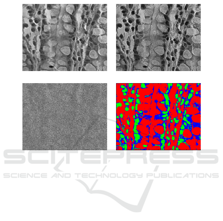
(a) (b)
no of peaks=3, used eig vecs=1234, epsilon=3, q levels=32
(c) (d)
Figure 1: A hyper-spectral microscopy image of a healthy human tissue. (a) The WAV of the original image. (b) The 50
th
wavelength. (c) The 95
th
wavelength. (d) The results of the application of the WWG algorithm with η(δ) = 4, θ = 3, ξ =
3, l = 32.
Segmentation of Hyper-spectral Microscopy Im-
ages. Figure 1 contains samples of healthy human
tissues and the results of the application of the WWG
algorithm on them. The images are of sizes 300 ×
300 ×128 and 151 ×151×128, respectively. The im-
ages contain three types of substances: nuclei, cyto-
plasm and glass. The glass belongs to the plate where
the tissue sample lies.
Figures 1(b) and 1(c) show the 50
th
and 95
th
wave-
lengths, respectively. The images in the 50
th
through
the 70
th
wavelengths are less noisy than the rest of the
wavelengths which resemble Fig. 1(c). Figures 1(d)
display the results after the application of the WWG
algorithm. The algorithm clearly segments this image
into three parts: the background is colored in dark
gray, the cytoplasm is colored in medium shaded gray
and the nuclei is colored in light gray.
Segmentation of Remote-Sensed Images. Figure
2 contains a hyper-spectral satellite image of the
Washington DC’s National Mall and the result after
the application of the WWG algorithm on it. The im-
age is of size 300 × 300 × 100. Figure 2(a) shows the
WAV of the image. The image contains water, two
types of grass, trees, two types of roofs, roads, trails
and shadow. Figures 2(b) and 2(c) show the 10
th
and
80
th
wavelengths, respectively. Figure 2(d) is the re-
sults of the WWG algorithm where the water is col-
ored in blue, the grass is colored in two shades of light
green, the trees are colored in dark green, the roads
are colored in red, the roofs are colored in pink and
yellow, the trails are colored in white and the shadow
is colored in black.
6 FUTURE RESEARCH
The results in section 5 were obtained using a Gaus-
sian kernel. It is shown in (Coifman and Lafon, 2006)
that any positive semi-definite kernel may be used for
the dimensionality reduction. Rigorous analysis of
families of kernels to facilitate the derivation of an
optimal kernel for a given set Γ is an open problem
and is currently being investigated by the authors.

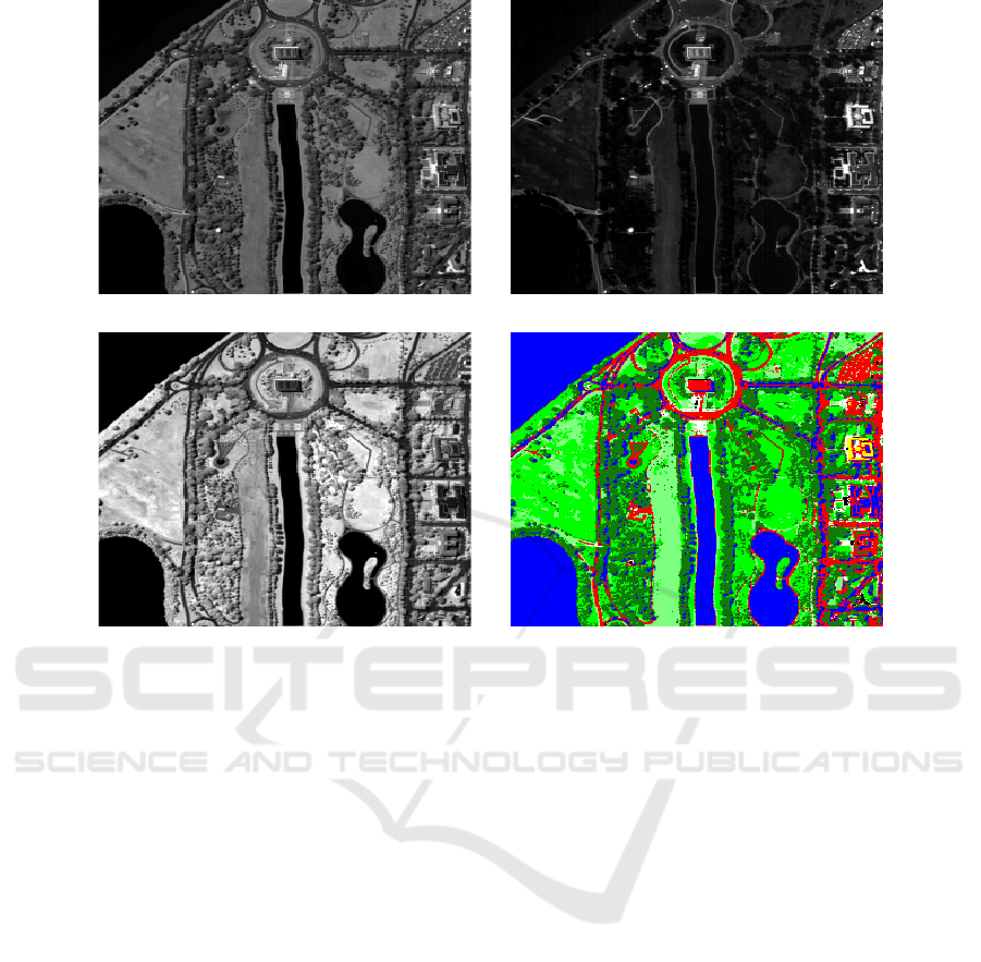
(a) (b)
(c) (d)
Figure 2: A hyper-spectral satellite image of the Washington DC’s National Mall. (a) The WAV of the image. The image
contains water, two types of grass, trees, two types of roofs, roads, trails and shadow. (b) The 10
th
wavelength. (c) The 80
th
wavelength. (d) The result after the application of the WWG algorithm using η (δ) = 4, θ = 8, ξ = 7, l = 32. The water is
colored in blue, the grass is colored in two shades of light green, the trees are colored in dark green, the roads are colored in
red, the roofs are colored in pink and yellow, the trails are colored in white and the shadow is colored in black.
The parameter η(δ) determines the dimensional-
ity of the diffusion space. Automatic choice of this
threshold is vital in order to detect the objects in the
image cube. A rigorous way for choosing η(δ) is cur-
rently being studied by the authors. Naturally, η(δ) is
data driven (similarly to choosing ε in (Schclar and
Averbuch, 2015)) i.e. it depends on the set Γ at hand.
REFERENCES
Bioucas-Dias, J. and Figueiredo, M. (2009). Logistic
regression via variable splitting and augmented la-
grangian tools. Technical report, Instituto Superior
Tecnico, TULisbon.
Cassidy, R. J., Berger, J., Lee, K., Maggioni, M., and Coif-
man, R. R. (2004). Analysis of hyperspectral colon
tissue images using vocal synthesis models. In Con-
ference Record of the Thirty-Eighth Asilomar Confer-
ence on Signals, Systems and Computers, volume 2,
pages 1611–1615.
Chan, T., Esedoglu, S., and Nikolova, M. (2006). Algo-
rithms for finding global minimizers of image seg-
mentation and denoising models. SIAM Journal Ap-
plied Mathematics, 66:1632–1648.
Coifman, R. R. and Lafon, S. (2006). Diffusion maps. Ap-
plied and Computational Harmonic Analysis: special
issue on Diffusion Maps and Wavelets, 21:5–30.
Li, F., Ng, M. K., Plemmons, R., Prasad, S., and Zhang,
Q. Hyperspectral image segmentation, deblurring, and
spectral analysis for material identification.
Li, J., Bioucas-Dias, J., and Plaza, A. (2010). Supervised
hyperspectral image segmentation using active learn-
ing. In IEEE GRSS Workshop on Hyperspectral Image
and Signal Processing, volume 1, pages 1–4.
Schclar, A. (2008). A Diffusion Framework for Dimension-
ality Reduction, pages 315–325. Springer US, Boston,
MA.
Schclar, A. and Averbuch, A. (2015). Diffusion bases di-
mensionality reduction. In Proceedings of the 7th In-
ternational Joint Conference on Computational Intel-
ligence (IJCCI 2015) - Volume 3: NCTA, Lisbon, Por-
tugal, November 12-14, 2015., pages 151–156.
Schclar, A., Averbuch, A., Hochman, K., Rabin, N., and
Zheludev, V. (2010). A diffusion framework for de-
tection of moving vehicles. Digital Signal Process-
ing,, 20(1):111–122.

Tarabalka, Y., Chanussot, J., and Benediktsson, J. A.
(2010). Segmentation and classification of hyperspec-
tral images using watershed transformation. Pattern
Recognition, 43(7):2367–2379.
Vincent, L. and Soille, P. (1991). Watersheds in digital
spaces: An efficient algorithm based on immersion
simulations. IEEE Transactions on Pattern Analysis
and Machine Intelligence, 13(6):583–598.
Ye, J., Wittman, T., Bresson, X., and Osher, S. (2010). Seg-
mentation for hyperspectral images with priors. In
Proc. 6th International Symposium on Visual Comput-
ing, Las Vegas, NV, USA., volume 1, pages 1–4.
Zheludeva, V., Polonena, I., Neittaanmaki-Perttuc, N.,
Averbuch, A., Gronroos, P. N. M., and Saari, H.
(2015). Delineation of malignant skin tumors by hy-
perspectral imaging using diffusion maps dimension-
ality reduction. Biomedical Signal Processing and
Control, 16:48–60.