Performance of Complex-Valued Multilayer Perceptrons Largely

Depends on Learning Methods

Seiya Satoh

and Ryohei Nakano

National Institute of Advanced Industrial Science and Tech, 2-4-7 Aomi, Koto-ku, Tokyo, 135-0064, Japan

Chubu University, 1200 Matsumoto-cho, Kasugai, 487-8501, Japan

Keywords:

Complex-valued Neural Networks, Complex-valued Multilayer Perceptron, Learning Method, Singular

Region, Singularity Stairs Following.

Abstract:

Complex-valued multilayer perceptrons (C-MLPs) can naturally treat complex numbers, and therefore can

work well for the processing of signals such as radio waves and sound waves, which are naturally expressed as

complex numbers. The performance of C-MLPs can be measured by solution quality and processing time. We

believe the performance seriously depends on which learning methods we employ since in the search space

there exist many local minima and singular regions, which prevent learning methods from ﬁnding excellent

solutions. Complex-valued backpropagation (C-BP) and complex-valued BFGS method (C-BFGS) are well-

known for learning C-MLPs. Moreover, complex-valued singularity stairs following (C-SSF) has recently

been proposed as a new learning method, which achieves successive learning by utilizing singular regions

and guarantees monotonic decrease of training errors. Through experiments using ﬁve datasets, this paper

evaluates how the performance of C-MLPs changes depending on learning methods.

1 INTRODUCTION

Recently the research on complex-valued neural net-

works have expanded in both quality and quantity

(Hirose, 2012). Complex-valued multilayer percep-

tron (C-MLP) can naturally treat complex numbers

and therefore can do function approximation in the

complex-valued world.

We evaluate the performance of C-MLPs by so-

lution quality and processing time. We believe the

performance greatly depends on learning methods

because in the search space there exist many local

minima and singular regions, which prevent learning

methods from ﬁnding excellent solutions.

Complex-valued backpropagation (C-BP) was

proposed (Nitta, 1997) as the ﬁrst learning method

of C-MLP. It performs search using only complex

gradient. Complex-valued BFGS (C-BFGS) (Popa,

2015) is a complex-valued version of quasi-Newton

method with the BFGS update (Nocedal and Wright,

2006). The performance of C-BFGS was reported

(Popa, 2015) to exceed those of other learning meth-

ods such as C-BP and Complex-valued Radial Basis

Function (C-RBF).

Recently a new learning method called Complex-

valued Singularity Stairs Following (C-SSF) has been

proposed. C-SSF performs search successively by in-

crementing the number of hidden units one by one

and inheriting an excellent solution from the previ-

ous learning through singular regions, and thus guar-

antees monotonic decrease of training errors. The

original version of C-SSF was proposed in (Satoh

and Nakano, 2014), but its search ability was lim-

ited and the learning speed was rather slow. Then

the search ability was enhanced and at the same time

the learning efﬁciency was greatly improved by in-

troducing search pruning and limiting the number

of search routes (Satoh and Nakano, 2015a)(Satoh

and Nakano, 2015b). The latest version (Satoh and

Nakano, 2015b) was used in this paper.

This paper shows how the performance of C-

MLPs depends on learning methods through exper-

iments using three quite different types of learning

methods and ﬁve different types of datasets.

This paper is organized as follows. First we intro-

duce the forward computation and singular regions of

C-MLPs in Section 2. Section 3 brieﬂy explains the

new learning method C-SSF together with two exist-

ing methods C-BP and C-BFGS. Section 4 shows ex-

perimental results obtained using three learning meth-

Satoh S. and Nakano R.

Performance of Complex-Valued Multilayer Perceptrons Largely Depends on Learning Methods.

DOI: 10.5220/0006496500450053

In Proceedings of the 9th International Joint Conference on Computational Intelligence (IJCCI 2017), pages 45-53

ISBN: 978-989-758-274-5

ods and ﬁve data sets together with considerations. Fi-

nally Section 5 concludes the paper.

2 COMPLEX-VALUED

MULTILAYER PERCEPTRON

2.1 Forward Computation

In this paper, C-MLP(J) denotes a complex-valued

MLP having J hidden units and a single output

unit. Weights {w

}, {w

}, input x

x, output f,

teacher signal y can be complex. A column pa-

rameter vector of C-MLP(J) is given below: θ

(J)



(J)

,··· ,w

(J)

,··· ,w

(J)



. Here w

(J)

is a column weight vector from input units to hidden

unit j, and w

(J)

is a scalar weight from hidden unit j

to the output. Moreover, a

denotes the transpose of

a. The output of C-MLP(J) can be shown as follows.

Here z

(J)

indicates the output of hidden unit j, and g

denotes an activation function.

x;θ

(J)

) = w

(J)

∑

j=1

(J)

, (1)

(J)

≡ g(w

(J)

x) (2)

In this paper we employ the following activation func-

tion (Kim and Guest, 1990; Leung and Haykin, 1991),

where c = a + ib and i =

√

−1.

g(c) =

1+ e

−c

1+ e

−a

cosb+ ie

−a

sinb

1+ 2e

−a

cosb+ e

−2a

(3)

When c is a real number, the function is the well-

known sigmodal one; however, here c is a complex

number, thus, the function can be transformed as

above, which means it gets periodic and unbounded.

We believethis nature plays an important role to allow

C-MLPs to have the ﬂexible capabilities for function

approximation.

Given training data {(x

),µ = 1,··· , N}, we

want to ﬁnd θ

(J)

minimizing an objective func-

tion. Our objective function is the following sum-of-

squares error, where

denotes the complex conju-

gate of δ

∑

µ=1

, δ

≡ f

;θ

(J)

) −y

(4)

2.2 Singular Regions

There are many singular regions in the search space

of C-MLPs, as is also true with real-valued MLPs.

A singular region can be deﬁned as a ﬂat continuous

area where the gradient is zero. Thus, any gradient-

based search method cannot move any more once it

enters in this region.

Singular regions can be generated using reducibil-

ity mapping from the optimum of C-MLP(J−1) to the

search space of C-MLP(J). Reducibility mapping can

be derived from the concepts of uniqueness and re-

ducibility of C-MLPs (Nitta, 2013).

Let the optimum of C-MLP(J−1) be

(J−1)

. Now

consider three reducibility mapping α, β, and γ,

and apply these mappings to the optimum of C-

MLP(J−1) to get the following

(J)

, and

(J)

≡ {θ

(J)

| w

(J)

= bw

(J−1)

, w

(J)

= 0,

(J)

= bw

(J−1)

j−1

(J)

(J−1)

j−1

for j=2,··· ,J} (5)

(J)

≡ {θ

(J)

| w

(J)

+ w

(J)

g(w

(J)

1,0

) = bw

(J−1)

(J)

= (w

(J)

1,0

,0,··· ,0)

(J)

= bw

(J−1)

j−1

(J)

(J−1)

j−1

for j=2,··· ,J} (6)

(J)

≡ {θ

(J)

| w

(J)

= bw

(J−1)

(J)

+ w

(J)

= bw

(J−1)

m−1

(J)

= w

(J)

(J−1)

m−1

(J)

= bw

(J−1)

j−1

(J)

(J−1)

j−1

for j ∈ {2,··· , J}\{m},

for m = 2, ··· , J} (7)

Then we have two kinds of singular regions as below.

(1) The intersection of

(J)

and

(J)

forms the singu-

lar region

(J)

αβ

where weight w

(J)

1,0

is free.

(J)

αβ

≡ {θ

(J)

| w

(J)

= bw

(J−1)

, w

(J)

= 0,

(J)

= (w

(J)

1,0

,0,··· ,0)

(J)

= bw

(J−1)

j−1

(J)

(J−1)

j−1

j= 2,··· ,J} (8)

(2) The other singular region is

(J)

, where m =

2,··· ,J. Weights w

(J)

and w

(J)

must satisﬁes the fol-

lowing.

(J)

+ w

(J)

= bw

(J−1)

m−1

(9)

Using a free variable q, we can rewrite the above as

follows.

(J)

= q bw

(J−1)

m−1

, w

(J)

= (1 −q) bw

(J−1)

m−1

(10)

3 LEARNING METHODS

3.1 Existing Learning Methods

As existing learning methods, we focus on two meth-

ods: a basic one and an excellent one.

Complex-valued backpropagation (C-BP) (Nitta,

1997) is the most basic learning method of C-MLP.

It carries out search using only the complex gradient.

There can be two ways of processing a step length:

ﬁxed or adaptive. When using the unbounded acti-

vation function such as eq.(3), a step length should

be adaptive, since a ﬁxed step length may guide the

search into undesirable directions. Since we employ

eq.(3) as the activation function, our C-BP always

adapts a step length doing line search.

The Quasi-Newton method requires only the gra-

dient at each iteration, but by measuring the changes

in gradients, it calculates the approximate of the in-

verse Hessian to make the method much better than

the steepest descent or sometimes more efﬁcient than

the Newton method (Nocedal and Wright, 2006). Al-

though there are several ways of approximating the

inverse Hessian, the BFGS update is considered to

work best. Complex-valued BFGS (C-BFGS) (Popa,

2015) is a complex-valued version of quasi-Newton

method with the BFGS update. The performance of

C-BFGS was reported to exceed those of other exist-

ing learning methods.

3.2 New Learning Method: C-SSF

A new learning method called Complex-valued Sin-

gularity Stairs Following (C-SSF) was recently pro-

posed, and then two kinds of modiﬁcations have been

done to signiﬁcantly improve its performance. The

latest version is shown in (Satoh and Nakano, 2015b).

C-SSF starts search from C-MLP(J =1) and then

gradually increases the number J of hidden units one

by one until the speciﬁed number J

max

When searching C-MLP(J), the method begins

with applying reducibility mapping to the optimum

of C-MLP(J−1) to get two kinds of singular regions

(J)

αβ

and

(J)

. Since the gradient is zero all over the

singular region, C-SSF calculates eigenvalues of the

Hessian to ﬁnd descending directions. Following the

direction of the eigenvector corresponding to a neg-

ative eigenvalue, the method can descend the search

space. After leaving the singular regions, the method

employs C-BFGS as a search engine from then on.

The processing time gets larger as the number J

of hidden units gets large. This is natural because

the number of search routes increases as J gets large.

To make C-SSF much faster without deteriorating so-

lution quality, the following speeding-up techniques

were introduced (Satoh and Nakano, 2015b).

One is search pruning. In the search, we often ob-

tain duplicate solutions. Considering that duplicates

are obtained via much the same search routes, we in-

troduced search pruning to speed up the method by

monitoring the redundancy of search routes. In the

search of C-MLP(J), search points are stored at a cer-

tain interval (100 steps in our experiments) and the

current search line segment is checked at the certain

interval to see if it is close enough to any of the previ-

ous search line segments. If the condition holds, the

current search route is instantly pruned.

The other is to set the upper bound S

max

on the

number of search routes. That is, the number of the

search routes for each C-MLP(J) is limited by S

max

To implement this, we calculate eigenvalues of all ex-

pected initial points on the singular regions. Then,

we pick up the limited number of negative eigenval-

ues in ascending order, and perform search using their

eigenvectors. We assume the larger convex curva-

ture at a starting point may suggest the better solution

quality at the end of the search.

4 EXPERIMENTS

We performed experiments to evaluate how the per-

formance of C-MLPs depends on learning methods

using three quite different types of learning methods

and ﬁve different types of datasets.

As learning methods, we employed C-BP, C-

BFGS, and C-SSF. As described previously, they per-

form search in quite different paradigms. Our C-BP

always calculates a reasonable step length in the di-

rection of the gradient. Both C-BP and C-BFGS run

100 times independently changing initial weights for

each J. As for C-SSF, the upper bound of search

routes S

max

was set to 100 for each J, the free param-

eters of singular regions were set as follows: w

(J)

1,0

−1, 0, 1 and q = 0.5, 1.0, 1.5.

The common learning conditions are mentioned

below. The number of hidden units was changed as

J = 1, ··· ,20. As for initial weights, real and imag-

inary parts of each weight were randomly generated

from the range of (0, 1). Each method was termi-

nated if the number of sweeps exceeded 1,000 or the

step length of line search was smaller than 10

−8

As datasets, we used the following ﬁve: the

Lorenz chaotic system, two artiﬁcial data, linear and

nonlinear channel equalizations. Every dataset was

normalized as shown below to make learning easier.

x ← x/max(abs(x)), (11)

y ← (y−mean(y))/std(y) (12)

Then, for two artiﬁcial data, small Gaussian noise

with zero mean and 0.01 standard deviation was

added to each part of every teacher signal in a dataset.

Training error and test error are shown as the fol-

lowing mean squared error (MSE).

MSE =

∑

µ=1

, δ

= f

−y

(13)

4.1 Experiment 1

The Lorenz system (Lorenz, 1963) is deﬁned by the

following equations.

= σ(y−x) (14)

= x(ρ−z) −y (15)

= xy−βz (16)

The system is known for having chaotic solutions

called the Lorenz attractor for certain parameter val-

ues and initial conditions. Here system parameters σ,

ρ, and β were set to be 10, 28, and 8/3 respectively.

The initial values of x, y, and z were set to be −10,

−10, and 30 respectively.

Our preliminary experiments showed that one-

step ahead prediction can be accurately realized by

using C-MLPs; thus, we estimate p

t+∆t

by using cor-

rect p

(≡ x

+ i y

) as input, where ∆t was set to be

0.05. Note that z

was used to generate data, but was

not used in our prediction model. Sizes of training

and test data were set to be N

= 500 and N

test

= 500.

Test data starts right after training data.

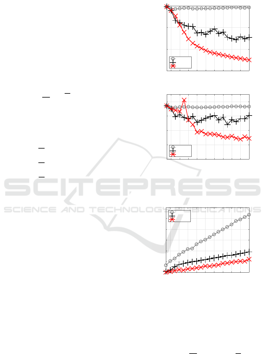
Figure 1 shows the smallest training MSE of each

method for each J. When J got larger, C-BP could not

decrease training error at all, C-BFGS could decrease

the error in a non-monotonic way, and C-SSF mono-

tonically decreased the error reaching the smallest.

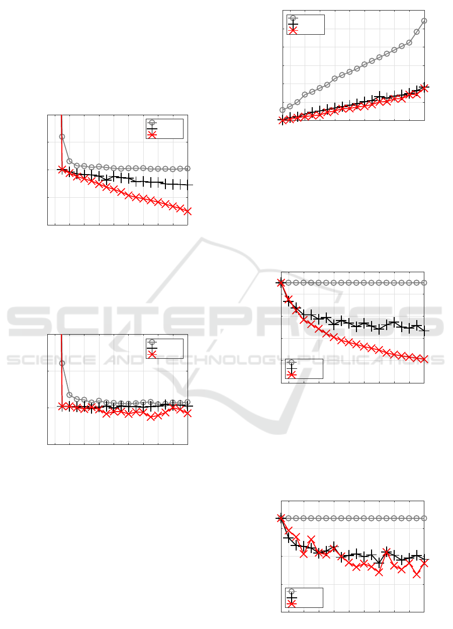
Figure 2 shows the smallest test MSE of each

method for each J. C-BP stayed at a high level, C-

BFGS showed smaller test errors than C-BP, and C-

SSF got better test errors than C-BFGS, showing the

smallest around high J.

Figure 3 shows CPU time required by each

method for each J. C-BP spent the largest time since

it could not converge spending maximum time, C-

BFGS was more efﬁcient and faster than C-BP, and

2 4 6 8 10 12 14 16 18 20

0.01

0.02

0.03

MSE

C-BP

C-BFGS

C-SSF1.3

Figure 1: Training errors for Experiment 1.

2 4 6 8 10 12 14 16 18 20

0.01

0.02

0.03

0.04

MSE

test

C-BP

C-BFGS

C-SSF1.3

Figure 2: Test errors for Experiment 1.

C-SSF was the fastest since it inherited an excellent

starting point for each J.

2 4 6 8 10 12 14 16 18 20

200

400

600

800

1000

1200

Processing time (sec)

C-BP

C-BFGS

C-SSF1.3

Figure 3: Processing time for Experiment 1.

4.2 Experiment 2

A complicated artiﬁcial dataset was generated using

the following function having four complex variables

and a reciprocal term. This dataset was used as a

benchmark (Savitha et al., 2009)(Popa, 2015).

f(z

) =

1.5



+ 10z



(17)

0.1 ≤|z

| ≤ 1, |z

| ≤ 1, k = 2,3,4 (18)

Sizes of training and test data were set to be N

3000 and N

test

= 1000.

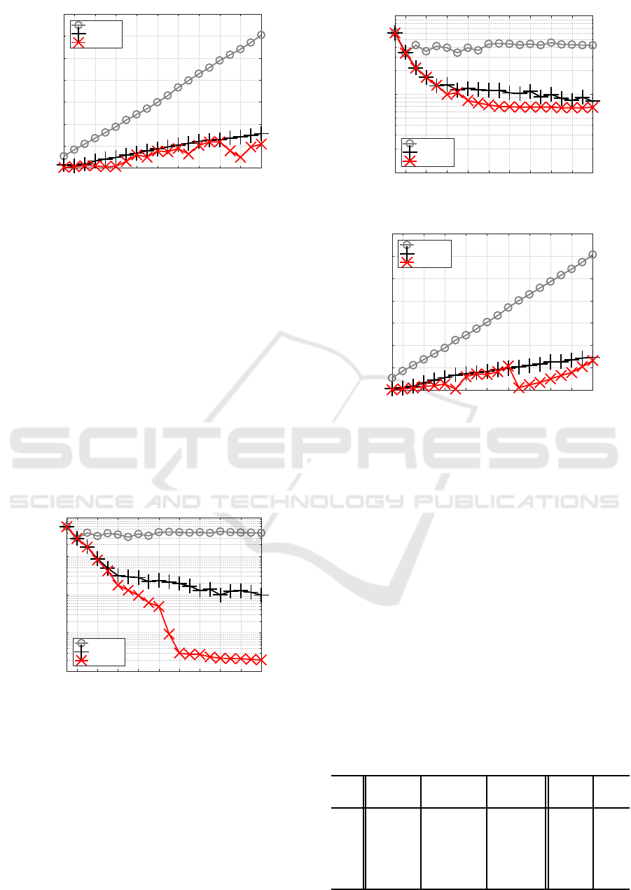
Figure 4 shows the smallest training MSE of each

method for each J. When J got larger, C-BP de-

creased training error with a limited amount only at

smaller Js, C-BFGS could decrease the error even fur-

ther in a non-monotonic way, and C-SSF monotoni-

cally decreased the error achieving the smallest.

2 4 6 8 10 12 14 16 18 20

0.01

0.02

0.03

0.04

0.05

MSE

C-BP

C-BFGS

C-SSF1.3

Figure 4: Training errors for Experiment 2.

Figure 5 shows the smallest test MSE of each method

for each J. C-BP decreased test error to some extent,

C-BFGS showed a bit smaller test error than C-BP,

and C-SSF got a bit better error than C-BFGS, show-

ing the smallest at J=15.

2 4 6 8 10 12 14 16 18 20

0.02

0.03

0.04

0.05

MSE

test

C-BP

C-BFGS

C-SSF1.3

Figure 5: Test errors for Experiment 2.

Figure 6 shows CPU time required by each method.

C-BP required the largest time, spending more as J

got larger, C-BFGS was more efﬁcient than C-BP, and

C-SSF was slightly better than C-BFGS.

4.3 Experiment 3

Another complicated artiﬁcial dataset was generated

using the following function having two complex

variables and treating separately the real and imagi-

nary parts. This dataset was also used as a benchmark

(Huang et al., 2008)(Popa, 2015).

f(z) = e

iIm(z)

(1−Re(z)

−Im(z)

) (19)

2 4 6 8 10 12 14 16 18 20

500

1000

1500

2000

2500

3000

Processing time (sec)

C-BP

C-BFGS

C-SSF1.3

Figure 6: Processing time for Experiment 2.

Sizes of training and test data were set to be N

3000 and N

test

= 1000.

Figure 7 shows the smallest training MSE of each

method for each J. When J got larger, C-BP could not

decrease training error at all, C-BFGS could decrease

the error to some extent in a non-monotonic way, and

C-SSF monotonically decreased the error obtaining

the smallest.

2 4 6 8 10 12 14 16 18 20

0.1

0.2

0.3

0.4

0.5

MSE

C-BP

C-BFGS

C-SSF1.3

Figure 7: Training errors for Experiment 3.

Figure 8 shows the smallest test MSE of each method

for each J. C-BP stayed at a high level, C-BFGS

showed much smaller test errors than C-BP, and C-

SSF got better test errors than C-BFGS, showing the

smallest around higher J.

2 4 6 8 10 12 14 16 18 20

0.1

0.2

0.3

0.4

0.5

MSE

test

C-BP

C-BFGS

C-SSF1.3

Figure 8: Test errors for Experiment 3.

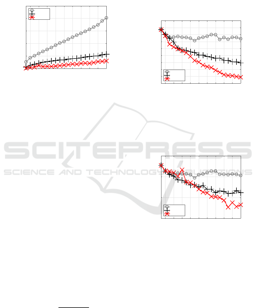
Figure 9 shows CPU time required by each method.

C-BP required the largest time, spending more as J

got larger, C-BFGS was much faster than C-BP, and

C-SSF was the fastest.

2 4 6 8 10 12 14 16 18 20

500

1000

1500

2000

2500

Processing time (sec)

C-BP

C-BFGS

C-SSF1.3

Figure 9: Processing time for Experiment 3.

4.4 Experiment 4

One important application of C-MLPs is in equaliza-

tion of quadrature amplitude modulation (QAM) of

complex-valued signals in linear or nonlinear chan-

nels. We consider 4-QAM linear channel equalization

(Chen et al., 1994)(Popa, 2015). The transfer function

of the linear channel was given as follows.

H(z) = (0.7409 −0.7406i)(1−(0.2−0.1i)z

−1

)

×(1−(0.6−0.3i)z

−1

) (20)

= 0.740900−0.740600i

−(0.296480−0.888840i)z

−1

−(0.022191+ 0.155562i)z

−2

(21)

The inputs to the channel were randomly generated

from the set s(k) = {±1 ±i}, and the output of the

channel was given as below.

∗

(k) = (0.740900−0.740600i)s(k)

−(0.296480−0.888840i)s(k−1)

−(0.022191+ 0.155562i)s(k−2)(22)

We observe the following o(k) including Gaussian

noise. Here n

(k) and n

(k) were generated from

Gaussian with zero mean and variance σ

o(k)= o

∗

(k)+n(k), n(k) ≡n

(k)+in

(k) (23)

Variance σ

was decided to make the following SNR

(signal-to-noise ratio) equal to 15 dB.

SNR = 10log



∑

k=1

∗

(k)|

∑

k=1

|n(k)|



(24)

Sizes of training and test data were set to be N

5000 and N

test

= 10000.

Figure 10 shows the smallest training MSE of

each method for each J. When J got larger, C-BP de-

creased training error only with a small amount in a

rather bumpyway, C-BFGS nicely decreased the error

as J got larger, and C-SSF monotonically decreased

the error even further achieving the smallest.

2 4 6 8 10 12 14 16 18 20

0.02

0.04

0.06

0.08

0.1

0.12

0.14

0.16

0.18

0.2

MSE

C-BP

C-BFGS

C-SSF1.3

Figure 10: Training errors for Experiment 4.

Figure 11 shows the smallest test MSE of each

method for each J. C-BP stayed around a high level,

C-BFGS decreased test error achieving smaller errors

than C-BP, and C-SSF got better test errors than C-

BFGS as J got larger, obtaining the smallest around

high Js.

2 4 6 8 10 12 14 16 18 20

0.05

0.1

0.15

0.2

MSE

test

C-BP

C-BFGS

C-SSF1.3

Figure 11: Test errors for Experiment 4.

Figure 12 shows CPU time required by each method

for each J. C-BP required the largest time, spending

more and more as J got larger, C-BFGS was much

faster than C-BP, and C-SSF was a bit faster than C-

BFGS.

4.5 Experiment 5

We consider complex-valued4-QAM nonlinear chan-

nel equalization (Savitha et al., 2009)(Popa, 2015).

The inputs to the channel were randomly generated

from the set s(k) = {±1±i}, and the output o

∗

(k) of

2 4 6 8 10 12 14 16 18 20

1000

2000

3000

4000

5000

6000

7000

Processing time (sec)

C-BP

C-BFGS

C-SSF1.3

Figure 12: Processing time for Experiment 4.

the channel was given as below.

∗

(k) = z(k) + 0.1z(k)

+ 0.05z(k)

(25)

z(k) = (0.34−0.27i)s(k)+(0.87+0.43i)s(k−1)

+(0.34−0.21i)s(k−2) (26)

We observe o(k) including Gaussian noise. The noise

level was set in the same way as in section 4.4.

o(k) = o

∗

(k) + n

(k) + in

(k) (27)

Sizes of training and test data were set to be N

5000 and N

test

= 10000.

Figure 13 shows the smallest training MSE of

each method for each J. When J got larger, C-BP

stayed at a high level, C-BFGS decreased the error to

some extent, and C-SSF monotonically decreased the

error achieving the smallest around high Js.

2 4 6 8 10 12 14 16 18 20

-5

-4

-3

-2

-1

MSE

C-BP

C-BFGS

C-SSF1.3

Figure 13: Training errors for Experiment 5.

Figure 14 shows the smallest test MSE of each

method for each J. C-BP stayed around a high level,

C-BFGS obtained much smaller errors than C-BP, and

C-SSF got a bit better test errors than C-BFGS, ob-

taining the smallest around high Js.

Figure 15 shows CPU time required by each

method. C-BP required the largest, spending more

as J got larger, C-BFGS was much faster than C-BP,

and C-SSF was a bit faster than C-BFGS.

2 4 6 8 10 12 14 16 18 20

-3

-2

-1

MSE

test

C-BP

C-BFGS

C-SSF1.3

Figure 14: Test errors for Experiment 5.

2 4 6 8 10 12 14 16 18 20

1000

2000

3000

4000

5000

6000

7000

Processing time (sec)

C-BP

C-BFGS

C-SSF1.3

Figure 15: Processing time for Experiment 5.

4.6 Considerations

Our experimental results are summarized focusing

on how the performance of C-MLPs depends on

learning methods. In more detail, we consider the

following: best training quality, average training

quality, generalization, processing time.

(1) Best training quality:

Table 1 shows the minimum training MSE of each

learning method for each dataset. For any dataset C-

SSF got the smallest, followed by C-BFGS and C-BP.

The ratio of C-BP to C-SSF indicates how many times

the minimum training MSE of C-BP is bigger than

that of C-SSF; it was between 2.0 and 1450. More-

over, the ratio of C-BFGS to C-SSF was between 1.6

and 49.

Table 1: Minimum training errors.

C-BP C-BFGS C-SSF ratio ratio

data

A B C A/C B/C

1 0.0286 0.0144 5.01e-3 5.72 2.87

0.0302 0.0245 0.015 2.02 1.64

3 0.449 0.234 0.107 4.22 2.20

0.143 0.0786 0.0376 3.80 2.09

5 0.0291 9.75e-4 2.00e-5 1450 48.7

(2) Average training quality:

Tables 2 and 3 show the average and standard devi-

ation respectively over 100 training MSEs of the op-

timal model (see Table 5) selected by each method

for each dataset. As for the averages, C-SSF achieved

the smallest for any dataset, followed by C-BFGS and

C-BP. The ratio of C-BP to C-SSF stretched between

1.7 and 2260, and the ratio of C-BFGS to C-SSF was

between 1.5 and 106. As for the standard deviations,

C-SSF achieved the smallest for most datasets, which

is reasonable since C-SSF always starts search from

good enough points.

Table 2: Averages over training errors of the optimal model.

C-BP C-BFGS C-SSF ratio ratio

data

A B C A/C B/C

1 0.0299 0.0221 5.84e-3 5.12 3.79

0.0325 0.0293 0.0194 1.68 1.51

3 0.450 0.330 0.114 3.95 2.90

0.164 0.0989 0.0443 3.69 2.23

5 0.0489 2.28e-3 2.16e-5 2260 106

Table 3: Standard deviations over training errors of the op-

timal model.

C-BP C-BFGS C-SSF ratio ratio

data A B C A/C B/C

1 8.28e-4 0.00212 6.59e-5 12.6 32.1

0.00131 4.31e-4 1.51e-4 8.68 2.85

3 1.52e-4 0.0340 9.49e-4 0.16 35.8

0.00794 0.00526 6.50e-4 12.2 8.08

5 0.00572 8.29e-4 0 Inf Inf

(3) Generalization:

Table 4 summarizes the minimum test MSE of each

method for each dataset. For any dataset C-SSF

achieved the smallest test MSE, i.e., the best gener-

alization, and C-BFGS got smaller test MSE than C-

BP. The ratio of C-BP to C-SSF spread out between

1.1 and 5.0, while the ratio of C-BFGS to C-SSF was

between 1.1 and 1.7.

Table 4: Minimum test errors.

C-BP C-BFGS C-SSF ratio ratio

data A B C A/C B/C

1 0.0359 0.0241 0.0139 2.59 1.74

2 0.0309 0.0298 0.0275 1.12 1.08

0.437 0.276 0.235 1.86 1.17

4 0.147 0.109 0.0769 1.91 1.42

0.0332 8.11e-3 6.68e-3 4.97 1.21

Table 5 shows the number of hidden units of the op-

timal model selected by each learning method for

each dataset. The optimal model indicates C-MLP(J)

showing the minimum test MSE. The table shows

how the optimal model differs depending on learning

methods.

Table 5: The numbers of hidden units of the optimal models

selected by learning methods.

data C-BP C-BFGS C-SSF

1 2 15 18

16 7 15

3 6 14 19

4 9 17 17

2 20 17

(4) Processing time:

Table 6 shows average numbers of training iterations

required by each learning method. For each dataset C-

BP reached the maximum iterations (sweeps), which

means C-BP was on the way in the search. For each

dataset C-SSF required the smallest number of itera-

tions until convergence. The ratio of C-BFGS to C-

SSF was between 1.7 and 3.6.

Table 7 summarizes total processing time (hr:

min: sec) of each method for each dataset. For any

dataset C-SSF was the fastest, and C-BFGS was faster

than C-BP. The ratio of C-BP to C-SSF spread be-

tween 3.7 and 7.4, while the ratio of C-BFGS to C-

SSF was between 1.2 and 2.3. The reason why C-

SSF was faster than C-BFGS may come from the fact

that the number of iterations required by C-SSF was

a few times smaller than that of C-BFGS. Besides,

the why C-BFGS was faster than C-BP in spite of its

higher complexity may be derived from the situation

that line search required by C-BFGS was much lighter

and faster than that of C-BP.

Table 6: Average numbers of training iterations.

C-BP C-BFGS C-SSF ratio ratio

data A B C A/C B/C

1 1000 937 291 3.44 3.22

2 1000 949 569 1.76 1.67

1000 940 264 3.8 3.57

4 1000 873 472 2.12 1.85

1000 890 338 2.96 2.64

Table 7: Total processing time.

C-BP C-BFGS C-SSF ratio ratio

data

A B C A/C B/C

1 3:28:53 1:17:38 0:38:34 5.42 2.01

7:37:25 2:28:14 2:02:14 3.74 1.21

3 6:17:17 1:57:55 0:50:55 7.41 2.32

17:56:38 4:47:45 3:12:59 5.58 1.49

5 18:03:17 4:38:47 2:43:39 6.62 1.70

5 CONCLUSIONS

The paper evaluated how the performance of C-MLPs

depends on learning methods. We employed three

quite different methods, C-BP, C-BFGS, and C-SSF,

and used ﬁve datasets. Performance was evaluated in

terms of minimum and average training errors, mini-

mum test error, and processing time. Our experiments

showed rather deﬁnite ordering: that is, at each evalu-

ation item C-SSF was the best, C-BFGS was the sec-

ond, and C-BP was the third. Although C-BFGS was

the best in most cases in (Popa, 2015), C-SSF was

not tried in the work. Moreover, the optimal models

selected by learning methods considerably differed

from each other. In the future we will investigatemore

using more datasets.

ACKNOWLEDGEMENTS

This work was supported by Grants-in-Aid for Scien-

tiﬁc Research (C) 16K00342.

REFERENCES

Chen, S., McLaughlin, C., and Mulgrew, B. (1994).

Complex-valued radial basis function network, part ii:

Application to digital communications channel equal-

isation. Signal Process., 36(2):175–188.

Hirose, A. (2012). Complex-Valued Neural Networks.

Springer, 2nd edition.

Huang, G.-B., Li, M.-B., Chen, L., and Siew, C.-K.

(2008). Incremental extreme learning machine with

fully complex hidden nodes. Neurocomput., 71:576–

583.

Kim, M. and Guest, C. (1990). Modiﬁcation of backpropa-

gation networks for complex-valued signal processing

in frequency domain. In Proc. IJCNN’90, volume 3,

pages 27–31.

Leung, H. and Haykin, S. (1991). The complex backprop-

agation algorithm. IEEE Trans. Signal Processing,

39(9):2101–2104.

Lorenz, E. (1963). Deterministic nonperiodic ﬂow. Journal

of the Atmospheric Sciences, 20(2):130–141.

Nitta, T. (1997). An extension of the back-propagation

algorithm to complex numbers. Neural Networks,

10(8):1391–1415.

Nitta, T. (2013). Local minima in hierarchical structures of

complex-valued neural networks. Neural Networks,

43:1–7.

Nocedal, J. and Wright, S. (2006). Numerical optimization.

Springer.

Popa, C.-A. (2015). Quasi-Newton learning methods

for complex-valued neural networks. In Proc. Int.

Joint Conf. on Neural Networks (IJCNN 2015), pages

1142–1149.

Satoh, S. and Nakano, R. (2014). Complex-valued mul-

tilayer perceptron search utilizing singular regions of

complex-valued parameter space. In Proc. Int. Conf.

on Artiﬁcial Neural Networks (ICANN 2014), pages

315–322.

Satoh, S. and Nakano, R. (2015a). Complex-valued mul-

tilayer perceptron learning using singular regions and

search pruning. In Proc. Int. Joint Conf. on Neural

Networks (IJCNN 2015), pages 1195–1200.

Satoh, S. and Nakano, R. (2015b). A yet faster version of

complex-valued multilayer perceptron learning using

singular regions and search pruning. In Proc. NCTA,

pages 122–129.

Savitha, R., Suresh, S., Sundararajan, N., and Saratchan-

dran, P. (2009). A new learning algorithm with loga-

rithmic performance index for complex-valued neural

networks. Neurocomputing, 72:3771–3781.