
Implementing a New Approach for Bidirectional Interaction between
a Real-time Capable Overall System Simulation and Structural
Simulations
Completion of the Virtual Testbed with Finite Element Analysis
Dorit Kaufmann, Malte Rast and Jürgen Roßmann
Institute for Man-Machine Interaction (MMI), RWTH Aachen University, Ahornstr 55,
52074 Aachen, Germany
Keywords: Rigid Body Dynamics (RBD), Finite Element Analysis (FEA), Virtual Testbed, Overall System Simulation,
Structural Simulation.
Abstract: Modern technical systems consist of various different components acting together. Robotics is a
sophisticated example, as mechanical and electrical components interact with the environment. With size
and complexity of the system, the susceptibility to errors rises, when the interaction between components
fails. Often this happens if a component shows minimal changes to the nominal function. The structural
behaviour of a single component is therefore as crucial for the functionality of the whole system as the
interaction of all components. Although sophisticated Overall System Simulations exist and create powerful
Virtual Testbeds, structural influences are neglected. As the underlying models differ, structural simulations
are used as a stand-alone tool and their results are barely considered in the overall picture. In this work an
interface was implemented, which is capable to integrate structural simulation automatically into a Virtual
Testbed framework.
1 INTRODUCTION
Today simulations are a cheap and fast way to test
the functionality of single construction components
or even whole systems. There are many different
methods engineers can use, depending on the
considered problem and the desired outcome. Rigid-
body dynamics (RBD) on the one hand is a
simulation technique where the dynamic behaviour
of a system of rigid bodies can be described. As it
assumes all parts to be non-deformable, it is quite
fast – even real-time capable for systems with
limited size. On the other hand, Finite Element
Analyses (FEA) take structural effects into account.
For this reason, they are quite slow, but provide
detailed results.
Usually it depends on the application which
simulation technique is chosen. But for many
complex questions the simplification of dividing the
whole system into subsystems is not appropriate, as
the interaction of the parts often determines the
behaviour of the whole complex. A good example
for this is the field of robotics. A robot consists of
multiple components which act in an electrical,
mechanical and structural manner altogether.
Consequently, the engineers of different disciplines
have to combine their knowledge. Therefore, an
interaction of the involved simulation programs is
crucial, which are combined in an Overall System
Simulation.
In this paper a new method is developed to
enable a bidirectional interaction between RBD and
structural simulations, where the RBD is already
integrated in the Overall System Simulation
framework. The new interface to the structural
simulations works completely automated. The
interaction is realized via a direct
force/displacement-exchange and implemented in
the environment of a Virtual Testbed. A Virtual
Testbed not only consists of the different
components of the Overall System Simulation, but
includes a simulation of the surrounding of the
technical system, a 3D-visualization and a graphical
user interface (GUI). This guarantees a wide range
of applications within an easy to use framework.
The precision of a structural simulation is
combined with the speed of RBD. The whole
114
Kaufmann, D., Rast, M. and Roßmann, J.
Implementing a New Approach for Bidirectional Interaction between a Real-time Capable Overall System Simulation and Structural Simulations - Completion of the Virtual Testbed with Finite
Element Analysis.
DOI: 10.5220/0006439301140125
In Proceedings of the 7th International Conference on Simulation and Modeling Methodologies, Technologies and Applications (SIMULTECH 2017), pages 114-125
ISBN: 978-989-758-265-3
Copyright © 2017 by SCITEPRESS – Science and Technology Publications, Lda. All rights reserved

simulation is validated on three levels. Both
simulation methods produce physically correct
results, which is proven by comparing a simulated
model with the according analytical calculation.
Even more important, the developed interaction
maintains the achieved level of accuracy and is
therefore qualified to complete the Virtual Testbed.
An example from space robotics shows the
benefits from this interaction, when results from
lightweight construction can be included into the
dynamic process of system tests based on a 3D-
simulation of the whole system.
2 RELATED WORK
The completion of an Overall System Simulation
with results from structural simulations is needed in
various application fields, as automotive
engineering, lightweight construction for aerospace
engineering, robotics, biomedical engineering and
many more. Nevertheless, there are only a few
working approaches, which is mainly caused by the
difficulty that both simulation methods have
completely different physical and mathematical
models. Furthermore, the interaction of an Overall
System Simulation and structural simulation is a
rather new field of research. Thus, all existing
solutions for the problem are either quite theoretical
and therefore not usable yet or specialized for a
certain application. The theoretical approaches deal
with different co-simulation strategies (Busch, 2012)
and have to develop sophisticated methods for
extrapolation (Stettinger et al, 2014) and the time
step management (Stettinger et al, 2013) of the
individual systems. Although these works provide
important contributions to the fundamental research
in the field of interaction between Overall System
Simulation and structural simulation, they cannot be
used for real-life applications due to the complexity
of the simulation models.
The second approach solves the problem of
interaction from a more phenomenological point of
view, i.e. an integration of structural results is
intended rather than a classical co-simulation. A
common way of doing so is to record the maximum
acting forces for one component during the Overall
System Simulation and perform a durability test
afterwards with a structural simulation (Kono et al,
2010; Chung and Kim, 2010). Another widespread
use of structural results can be seen when it comes to
unwanted vibrations in technical systems. A modal
analysis helps to examine effects that cannot be seen
in an Overall System Simulation (Wang and Mills,
2004). Especially automotive and aerospace
engineering show a huge effort to include structural
results into an Overall System Simulation (Dietz,
Hippmann and Schupp, 2001; Wellmer, 2014).
In conclusion, combining both simulation
methods faces the problem that an application-
independent interaction needs sophisticated
mathematical models and underlying algorithms,
which lead to programs only usable for simple
scenarios. In case of a phenomenological approach,
a more complex model may be analysed, however,
the used interaction is limited to the special test
scenario.
Furthermore, all approaches have huge problems
with real-time capability.
3 KEY METHODS
The integration of structural simulations into a
Virtual Testbed framework is challenging due to
completely different workflows for both simulation
methods. The FEA is rather sophisticated and should
be done by an expert while the Virtual Testbed itself
must be easy to use. Nevertheless, the underlying
algorithms of RBD are complex as well. The
workflow of a FEA is integrated in the mathematical
model of RBD, thus both key methods are
explained.
3.1 FEA
The FEA is a standard method to calculate structural
deformations, i.e. get the behaviour of a component
due to outer influences like force or thermal load.
These relations are described by differential
equations in continuum mechanics. To handle the
problem numerically, a deformable component is
segmented into a large number of single elements.
This procedure of discretization is called meshing.
Every element has a characteristic number of edges
and nodes that connects it with neighbouring
elements. An initial function is assigned to every
element to describe its behaviour in the mesh. For
getting an overall solution, two conditions must be
fulfilled: the outer forces acting on the component
have to be completely transferred in deformation
energy and the elements have to keep their
connections to their neighbours. If both is true, the
simulation converges and the structural deformation
results of an integration of all elemental initial
functions. Mathematically, this is described by the
equation of elasticity for m elements, where
is the
Implementing a New Approach for Bidirectional Interaction between a Real-time Capable Overall System Simulation and Structural
Simulations - Completion of the Virtual Testbed with Finite Element Analysis
115

displacement of the elemental nodes in element i and
is the corresponding acting force.
(1)
The matrix includes the overall stiffness and
basically consists of elastic moduli. A detailed
mathematical description can be found in many text
books (Rieg and Steinhilper, 2012). Prior to solving
the above equation, boundary conditions (BC) have
to be defined, i.e. a defined behaviour for some
nodes has to be prescribed. This corresponds to
including supports, while the acting forces are called
loads. The procedure of meshing the component,
defining BC and thus the setup of an FEA is called
preprocessing. In the next step, algorithms solve the
equations using approximations. The allowed degree
of approximation is defined during the preprocessing
as well. If large errors are accepted, the simulation
loses its realistic representation, too small errors
result in a non-converging solution, as the meshes
usually become rather large and the solver is not
capable to fulfil the conditions. Thus, preprocessing
requires a lot of expertise and experience. In general,
the setup of an FEA has to be done several times,
before a realistic, converging solution can be
achieved. The solving itself is done by the solver
automatically and can last from a few seconds up to
several days. After a successful solving, the results
have to be verified, which is done during the
postprocessing.
3.2 RBD
RBD is used in the Virtual Testbed framework to
describe the dynamic interaction of multiple rigid
bodies (RB). The specific inertia tensor, centre of
mass and a collision hull is assigned to every RB. Its
active behaviour due to external forces
or
connections to other RB is calculated. The latter one
is considered by introducing constraint forces
, where is a Lagrangian Multiplier and
points in the direction of the constraint force. As the
constraint force forbids movement in a certain
direction, it has to act perpendicular to the
directions, where movements are allowed. Thus, a
so-called holonomic constraint applied to the
velocity
rather than the direction itself can be
written with a constant .
(2)
The constraint force has to be added in the
Newtonian axiom, which leads to the Lagrange
equation.
(3)
Given that the constraint is formulated in a
velocity rather than an acceleration space, the same
should apply for the Lagrange equation, which
finally leads to a more performant momentum-based
approach (Stewart and Trinkle, 2000). Using a
simple integration
(4)
with being the time step, one gets:
(5)
This is combined with the holonomic constraint
to a Linear Complementary Problem (LCP), which
can be solved by various algorithms (Jung, 2011).
(6)
4 CONCEPT
The general idea of the integration of structural
simulations into a Virtual Testbed framework is a
bidirectional interaction. The implemented interface
sends forces and momentums acting on a
component in the Virtual Testbed to the structural
simulation and gets back the resulting structural
bending, i.e. translations and rotations . This
concept of a direct variable exchange is visualized in
Figure 1.
Figure 1: Automated interaction of the Virtual Testbed
framework and structural simulation by a bidirectional
exchange of the characteristic variables.
Virtual Testbed framework
Structural simulation (FEA)
Interface,
Variable exchange
s
F
Master
(access point)
SIMULTECH 2017 - 7th International Conference on Simulation and Modeling Methodologies, Technologies and Applications
116

4.1 Requirements for a Functional
Interface
Two main aspects were identified as crucial for an
efficient interaction between a Virtual Testbed
framework and structural simulations:
1. Start a structural simulation only when really
needed.
2. Design a completely automated interface,
which at the same time assures retaining the
accuracy of both simulation methods.
The first point accounts to the fact that a
structural simulation is time-consuming and
provides a level of detail only needed in critical
situations, e.g. when a structure experiences
maximum load. The second point describes the
demand of a separation of expertise: both simulation
methods are rather sophisticated and should be set
up by experts. This is vital to assure that the
combined complex system simulation does not lose
validity and thereby its eligibility. At the same time,
the interaction has to take place in a framework easy
to use to give its full potential to the end-user.
Both mentioned prerequisites are considered in
the general concept of this interaction. It is
implemented in the Virtual Testbed framework, so
the user has the choice to complement the Virtual
Testbed with a structural simulation if needed.
Therefore the component whose structure should be
included is defined beforehand. The model is
divided in the deformable and the rigid part (see
Figure 2). A pure structural simulation is performed
with the deformable part, uncoupled to the Overall
System Simulation. Thus, the complex steps of a
FEA can be done by a different person, i.e. a FEA
engineer. Particularly meshing the component and
setting the solver parameters are crucial for the
realistic outcome of a structural simulation and
require a huge level of experience. Once the quality
of the setup for this specific structural simulation is
assured, it can be integrated into the Virtual Testbed.
To make sure that every case scenario in the
Virtual Testbed can be accounted for, the input file
of the structural simulation is parametrized. Like
this, all forces and momentums acting on the
component during a Virtual Testbed simulation can
be given to a structural simulation. The interface
deals with transmitting the actual values, starting a
new structural analysis, obtaining the desired results
and putting them back into the Virtual Testbed.
4.2 Model Division by a One-Side Joint
From the Overall System Simulation, the RBD part
is most valuable for the interaction with structural
simulations as it calculates the acting forces and
momentums on each component. This is done by
determining the constraint forces/momentums that
occur in the RB. By definition, the forces act on the
centre of mass, while the momentums are applied to
their point of action. Coming to the integration of
structural simulations, this causes a problem, as the
interaction between single components and therefore
the transmission of force happens at random points
on the surface. Thus, a new method is needed to get
the required variables at the division point of the
model, where the rigid and the deformable part
meet, out of the RBD equations. More precisely, in
order to calculate the acting forces and momentums,
a so-called one-side joint was implemented.
The general construct of a joint handles the
constraint forces at the meeting point of two RB, so
it is crucial to define and solve the Lagrangian
equations. Descriptively, the mathematical model
uses the joint frames and ensures that both sides
keep the geometric conformity, i.e. that the RB are
not separated. For the easiest example of a joint with
no degree of freedom, has to be a matrix with 6
rows and columns, while . Thus, the velocity-
based constraint has the following form, where
are translational/rotational velocities:
(7)
This equation finally leads to the constraint
force. It consists of the intrinsic acting force on the
component that occurs from its interaction with
other components. Thus, this force is needed for a
structural simulation of the corresponding
deformable part. Joints in general are an important
element of the RBD and therefore efficient
algorithms to solve the underlying equations already
exist. As the deformable component is not present in
the RBD anymore, the one-side joint misses a
counterpart. To get the right results and use more
sophisticated concepts like stabilization, the one-side
joint considers the starting pose of the joint frame on
the rigid part of the division point as a counterpart.
Thus, this joint fixes the rigid part at this point in
space, where usually the deformable part would be.
Implementing a New Approach for Bidirectional Interaction between a Real-time Capable Overall System Simulation and Structural
Simulations - Completion of the Virtual Testbed with Finite Element Analysis
117
To ensure a general validity of the equations to
solve, it has to be accounted for that different
coordinate systems (CS) can be used for the joint
frame and the RB frame in the centre of mass. With
describing the vector between those CS and
being the joint x-axis in the CS of the
RB, finally the corresponding constraint equation to
solve is
(8)
with , , , being 3x3-Matrices of the form
(9)
Further details on constraint equations in general
and the mathematical models used to implement
joints can be found in (Jung, 2011). By solving the
Lagrangian equation, one finally obtains the
constraint forces and momentums that act on the
division point of rigid and deformable part. The
interface automatically extracts those values and
initializes a new structural analysis with the acting
forces and momentums. When the FEA calculations
have finished, the interface extracts the resulting
translations and rotations of the division point. In
the next step, the whole RB system in the Virtual
Testbed is updated to the new pose caused by the
structural displacement of the deformable
counterpart. The whole interaction process is
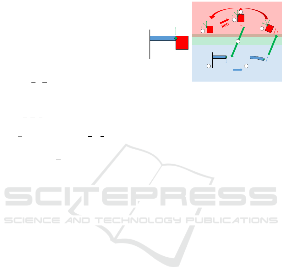
visualized in Figure 2 with the easy example of a
bar. It is fixated on the wall at one side, while the
other side is attached to a heavy load. Naturally, the
bar experiences bending, which can now be included
with the interface to structural simulation.
Figure 2: Integration of structural simulation into a Virtual
Testbed. The example shows a bending bar to visualize the
general workflow.
4.3 Limitations
The fact that a pure structural simulation is needed
in the first place may be considered as a restriction
to the general usability of the interaction. However,
it should be quite clear in a model which component
is likely to experience a structural deformation.
Furthermore, doing a sophisticated FEA before
allowing interaction allows the same separation of
expertise for models and algorithms as it does for
users, i.e. the functionality of the Virtual Testbed is
increased while efficiency is not reduced.
Another limitation lies in the visualization of the
deformable part in the Virtual Testbed. The
deformed shape cannot be imported yet, thus the
non-deformed starting shape is kept.
5 IMPLEMENTATION AND
DATAFLOW
The general concept of the interaction can be
implemented basically with any FEA and Virtual
Testbed framework. Nevertheless, some software is
more appropriate than other due to its usability,
accuracy or general functionality. The interface
combines both simulation methods using algorithms
running completely automated. The only task for the
end-user is to choose between different working
modes using the GUI of the Virtual Testbed
framework software.
5.1 Used Software for the Virtual
Testbed and FEA
For this work, the FEA part was done with ANSYS
Mechanical R 16.2 of ANSYS, Inc. Canonsburg,
Pennsylvania. It was favoured because of its
Division point
RigidDeformable
Interface
Virtual Testbed framework
F
Structural simulation
F
s
FEA
User request:
Start FEA
43
2
1
5
no
FEA
a
b
SIMULTECH 2017 - 7th International Conference on Simulation and Modeling Methodologies, Technologies and Applications
118
usability and accuracy, but the general concept of
the interaction works as well for different software.
The workflow for the FEA used for interaction is
shown in Figure 3. As described above, the model is
divided into a deformable and a rigid part first. A
FEA expert should do the setup of the structural
simulation for the deformable part. This can be done
in a usual manner, i.e. using the GUI of ANSYS.
After the validity of the structural analysis is assured
once, it is necessary to create a script to start the
solver with the very same setup again using an
ANSYS Parametric Design Language (APDL)-
Script. The given forces and momentums in the
script need to be parametrized manually. This takes
about 5 minutes and can be done with the help of a
manual that was written during this work. To start
the FEA solver without using the ANSYS GUI
again, a PreFile written in python is needed. In
general, it executes the APDL-Script and more
importantly for the FEA, it handles in- and output of
the FEA. Thus, for every requested FEA out of the
Overall System Simulation, the values of the actual
acting forces and momentums are assigned to the
parameters and the resulting translations and
rotations are extracted. This whole dataflow happens
completely automated, the end-user only has to
provide the APDL-Script and the GeneralPreFile
once. The interface generates all other files itself and
stores them in a self-built folder structure. This is a
significant part of the separation of expertise, as in
case a FEA fails to converge, all files for
troubleshooting can be sent to the FEA expert again.
Figure 3: Dataflow to create a parametrized FEA setup
that can be performed automatically by the interface.
For the Virtual Testbed, it is crucial to have a wide
range of functionalities and a framework the
interaction can be implemented in. The software
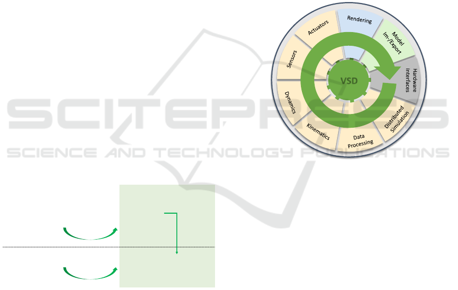
VEROSIM (Roßmann et al, 2013) meets both
requirements. It is based on a microkernel called
Versatile Simulation Database (VSD, see Figure 4).
This central structure handles the simulation models
and manages basic communication and meta
information. The whole software is object-oriented
and written in C++. That makes it possible to expand
the VSD by various special functionalities that are
integrated as plugins or extensions and finally allow
simulating a wide range of different applications.
Thus, different components of the Virtual Testbed
are not just simulated simultaneously, but rather in
the same environment what allows to consider
explicitly the influence they have on each other.
Finally the simulation is real-time capable and
rendered in 3D (Roßmann et al, 2013). Specialized
on eRobotics, VEROSIM is capable to simulate the
dynamic and kinematic behaviour of a robot together
with possible sensors or control algorithms and the
environment the robot is in. The integration of
structural simulation is an additional feature that
allows to simulate even more realistic situations in
robotics.
Figure 4: The VSD microkernel of VEROSIM (Roßmann
et al, 2013).
5.2 Modes of Operation
Finally, the user of the Virtual Testbed framework
can choose between two different working modes
for starting a new, completely automated operating
FEA out of the given RBD situation. Single buttons
in the underlying GUI of VEROSIM represent all
options.
1. DirectFEA (Figure 5): The RBD
simulation stops and the interface initializes a FEA
with the acting forces and momentums .
2. LazyModeFEA (Figure 6): Forces and
momentums are saved automatically while RBD
goes on. Using this mode, the time-consuming FEA
can be performed to a later point in time, e.g. over
night. Besides, the user of the Virtual Testbed
framework is capable to define his own forces to be
put into a FEA without dealing with the FEA
software itself. LazyModeFEA consists of several
APDL-Script
ANSYS Parametric Design Language
(Mechanical Solver)
• Parametrization of forces
GeneralPreFile
python
• Mask to execute
the script
• Regulates the
output of ANSYS
PreFile
python
• With acting
forces
ANSYS Workbench
GUI
• Setup structural
simulation
Files for interaction
Reference,
Execution
Specification
Creation
Pure FEA
VSD
Implementing a New Approach for Bidirectional Interaction between a Real-time Capable Overall System Simulation and Structural
Simulations - Completion of the Virtual Testbed with Finite Element Analysis
119
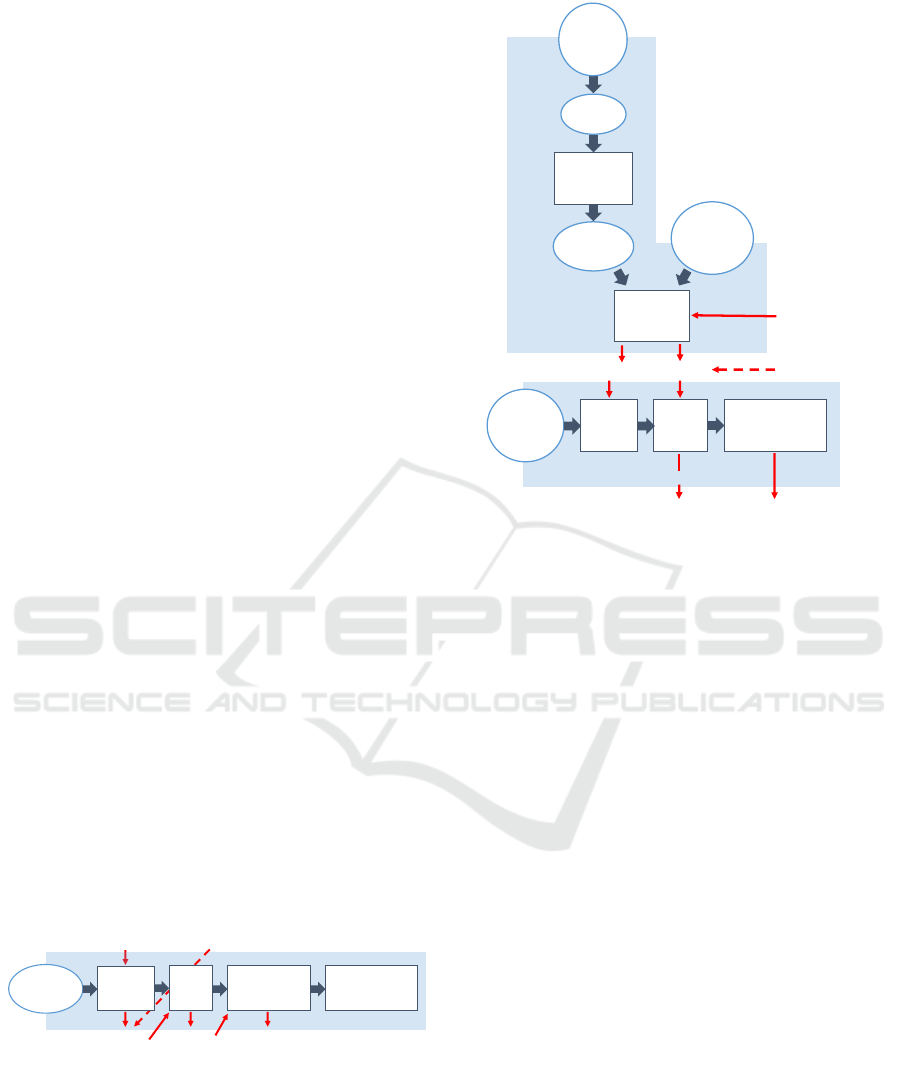
operating modes (LM_).
a. LM_direct: The actual acting forces and
momentums are saved.
b. LM_max: When activated, this mode
filters the maximum forces/momentums in each
direction during the whole simulation. It can be used
to decide whether structural deformation have an
unneglectable influence in the given model.
c. LM_start: Start FEA calculations for all
saved situations.
After each calculation, the given input- and
resulting output-values of each FEA are put into
lookup-tables, i.e. to each set of forces and
momentums a set of translations and rotations is
assigned. Thus, a database for each structural
simulated component is build up in the background.
If this database is profound enough, it becomes
possible to interpolate the phenomenological
structural behaviour of a component. By nature, this
interpolation is a transformation from one 6D space
(of forces and momentums) to another 6D space (of
translations and rotations). To handle the size of this
problem, two main simplifications were made. On
the one hand, all dimensions of deformation shall be
independent. On the other hand, the principle of
straight direction influence is introduced, i.e. to get
the translation in x-direction, only force in x- and
momentum in y- and z-direction are considered.
Taking those assumptions, the interpolation is from
3D to 4D. Delaunay triangulation is an
acknowledged way to deal with such a problem. To
try the validity of the general idea in an
uncomplicated way, the software MATLAB by The
MathWorks, Inc. Natickk, USA was integrated into
the Virtual Testbed framework. On user request, the
function griddata is called automatically with the
actual values. The computing time of the underlying
algorithm is below 1s and hence much faster than a
FEA.
Figure 5: Flow chart of the operation mode DirectFEA.
Round boxes are buttons in the GUI to start the working
modes, the outer descriptions are used/generated files of
the interaction, which works completely automated
(shaded area, rectangular boxes refer to crucial functions).
Figure 6: Flow chart of the operation mode
LazyModeFEA (see Figure 5 for explanation).
6 VALIDATION
An interaction between two simulation methods
requires a validation on three different levels: Each
method has to provide correct physical results
separately and furthermore it has to be assured this
accuracy is maintained during the interaction
process.
Especially for the Overall System Simulation,
this proposition is crucial. Several components
interact with each other and the environment,
thereby forming the Virtual Testbed. Adding a
certain aspect to the Overall System Simulation and
thus integrating a new simulation method (like RBD,
electrical or sensor simulation etc.) requires the three
defined validation steps. The software VEROSIM is
validated in the aforementioned way by comparing
simulated results to real world experiments
(Roßmann et al, 2013).
FEA is an acknowledged and well-described
simulation method to obtain structural deformations
(Bathe, 1996). Nevertheless, the complexity of the
method and its wide range of applications require a
validation for each new use case. As described
above, convergence and physical correctness is
checked by the FEA engineer during the
Direct
FEA
F
read
Displacem.
updatePose
(all RB)
General
PreFile
APDL-Script
PreFile
logFile,
errorFile
FEAlook-
upTables
start
FEA
write
PreFile
given by user
generated
automatically
VEROSIM Framework
read
Displacem.
LM_
start
Jobs
ToDo
start
FEA
VEROSIM
Framework
PreFileToDoList
write
PreFile
save
BiggestF
Run
RBD
LM_
max
F
Rest/
Stop
LM_
direct
F
generated
automatically
logFile,
errorFile
FEAlook-
upTables
given by user
General
PreFile
APDL-Script
VEROSIM Framework
SIMULTECH 2017 - 7th International Conference on Simulation and Modeling Methodologies, Technologies and Applications
120
postprocessing. An elaborated model was used to
prove the expertise of setting up a FEA correctly
before starting an interaction with the Overall
System Simulation. The model consists of a spring
on a steering between two plates and is compressed
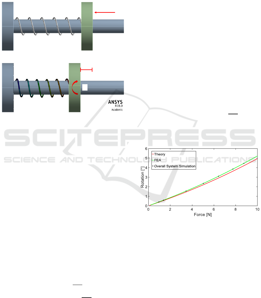
by an external force (see Figure 7).
Figure 7: Validation model of the interaction: a) A helical
spring on a steering is loaded with an external force . b)
The load leads to a deformation which can be described
with a compression and a rotation .
This example was chosen because the deformation
can be translated into a defined movement that can
be described analytically. Furthermore, it combines
two movements with a different range of
complexity: First, there is the compression itself,
which is described by the linear spring constant .
On the other hand, the spring will rotate around a
certain angle due to its helical shape. This
correlation is rather sophisticated (see equation
(14)). A spring with defined manufacturing
parameters was modelled (see Table 1) and loaded
with a force up to in the FEA. The underlying
mathematical models and data used in the analysis
can be found in the APPENDIX. The structural
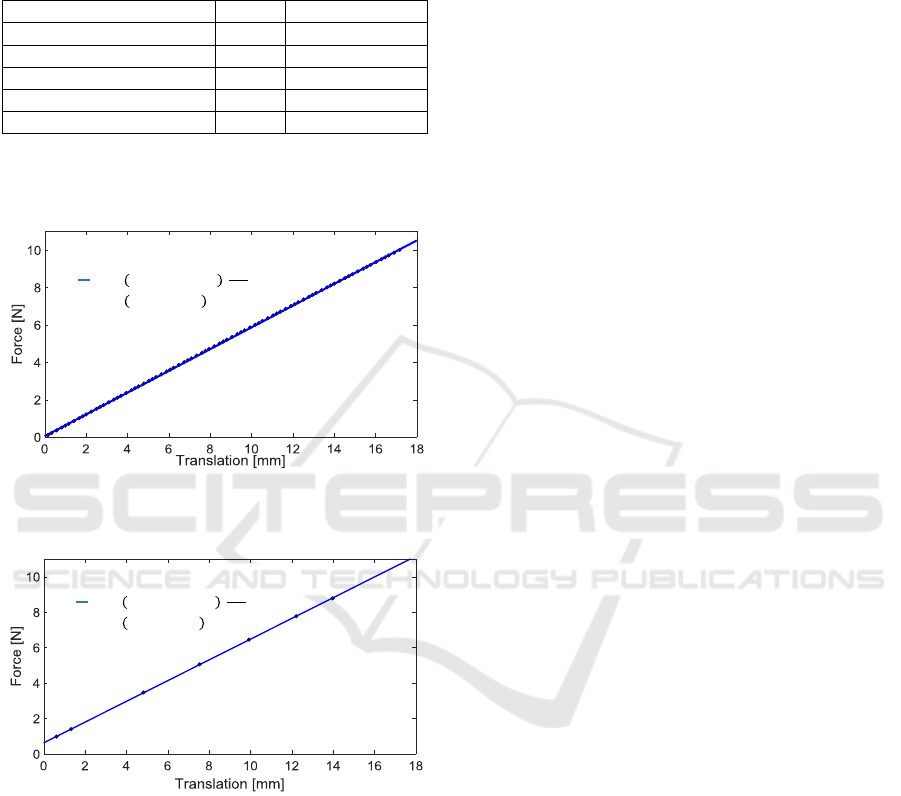
results are compared to the analytical ones. The
simulated spring constant is determined with a linear
regression (see Figure 11) and compared to the
analytical calculated one (see equation (13)):
(10)
The difference between the two results can be
explained by numerical errors in the FEA. However,
a deviation of is in the usual range of errors
for a FEA.
The simulated rotation is directly compared to
the analytical results (green and red lines in Figure
8) and shows a sensible accordance. Thus, the FEA
itself is capable of providing realistic results in every
sense for the given model of a spring.
The last validation step has to prove that the
interaction process does not decline the achieved
levels of accuracy of the FEA and the Overall
System Simulation. Hence, the spring was modelled
and loaded in a Virtual Testbed and the bidirectional
interaction was enabled. Thus, the acting forces and
momentums are calculated by RBD, a new FEA is
started and the model in the Virtual Testbed changes
its pose due to the structural deformation. The
position and orientation of the upper plate connected
to the spring were measured during different load
cases in the Overall System Simulation. Similarly to
the aforementioned analysis, the spring constant was
calculated with a linear regression (see Figure 12).
The result is the same as the one of the FEA:
(11)
The same holds true for the rotation. The results
in the Overall System Simulation reflect exactly the
structural results of the FEA (dots in Figure 8).
Figure 8: Rotation of the compression spring: the
analytical model, FEA and the Overall System Simulation
show the same results.
The three-level validation proves that both FEA and
the Overall System Simulation framework as well as
the developed bidirectional interaction are capable
of producing physically correct results. Hence, the
completed Virtual Testbed can be used in the future
to simulate a real-life scenario and define design
rules or guidelines for the tested applications.
a)
b)
Implementing a New Approach for Bidirectional Interaction between a Real-time Capable Overall System Simulation and Structural
Simulations - Completion of the Virtual Testbed with Finite Element Analysis
121
7 APPLICATIONS
Robotics is a field of research where not only
different components, but also different disciplines
have to work together to guarantee an overall
functionality. An actual example from space robotics
is taken to show the features and usability of the
developed interaction: While monolithic satellites
lose their purpose if one of the components is
broken, the project iBOSS builds satellites out of
single blocks that can be assembled and
reconfigured in space (Weise et al, 2012). This
modular structure has completely new requirements
for the used materials. However, even defining those
requirements is a difficult task, as the workflow
between materials science and mechatronics faces a
vicious circle here: The loading conditions are
analysed when choosing a material to ensure the
durability of the component is appropriate. The
acting loads are caused by another component, e.g. a
robot moving to perform a certain task.
Simultaneously, the movement of the robot itself
will be influenced by structural effects occurring in
the first component. This problem cannot be solved
without a sophisticated analysis of the interaction
between structural simulations and the Overall
System Simulation. To show the functionality of the
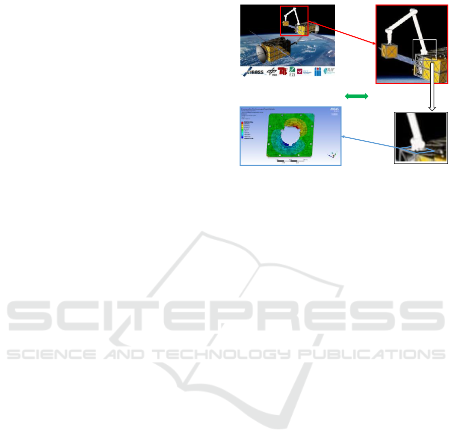
developed interface in a similar use case, a
lightweight robot was fixed onto one of the iBOSS
building blocks.
The division point in the model is defined at the
fixation between the robot and the building block.
The robot stays in the Virtual Testbed and its
movements are calculated using RBD. The plate of
the building block where the robot is fixated is
defined as the deformable part and hence undergoes
structural analyses (see Figure 9). After the setup of
this specific FEA has been done by an expert and
convergence was achieved, the interface can be
used. In the Virtual Testbed, the robot moves in a
defined way, like it would to complete a certain task.
On user request, the actual forces acting on the plate
are sent to ANSYS and a new FEA is done. The
resulting deformations of the plate are recorded,
averaged over the whole section of the plate and the
base of the robot and all the connected RB are
updated to the new pose. After the update, RBD
continues and any influences on the robot’s
movements due to the slightly different pose are
accounted for.
Figure 9: Application scenario for the implemented
interaction: the modelling of the lightweight robot happens
in the Virtual Testbed. Its movements cause structural
deformations of the plate it is fixated on, which are
directly included in the Virtual Testbed.
The presented example was only performed as a
feasibility study, i.e. the used material for the plate is
not the final one and the robot will not be fixated
with simple screws, as it was done in this study.
Nevertheless, it should be clear that the developed
interaction works and more sophisticated
simulations can be performed in exactly the same
way.
The same is true for the functionality of the
interpolation method. It should be used carefully as a
non-adequate database may lead to wrong results.
Nevertheless, a first feasibility study with the same
example of the robot on a plate shows that the
approach can reproduce FEA results quite
accurately. Therefore, the movements of the robot
and the resulting forces and momentums were
recorded during a certain period of time (see Figure
10a). The resulting deformations averaged over the
whole plate were calculated with the interpolation
method and compared to a directly performed FEA
with the same input values (Figure 10b). The only
significant deviations appear in z-direction, where
deformations barely occur. The scale of deformation
is more than ten times smaller than in the other
directions. Thus, the interpolation deals with values
around zero, which do not show a clear amplitude
and therefore have a bigger variety.
Virtual Testbed
framework
Structural simulation
Interface
SIMULTECH 2017 - 7th International Conference on Simulation and Modeling Methodologies, Technologies and Applications
122
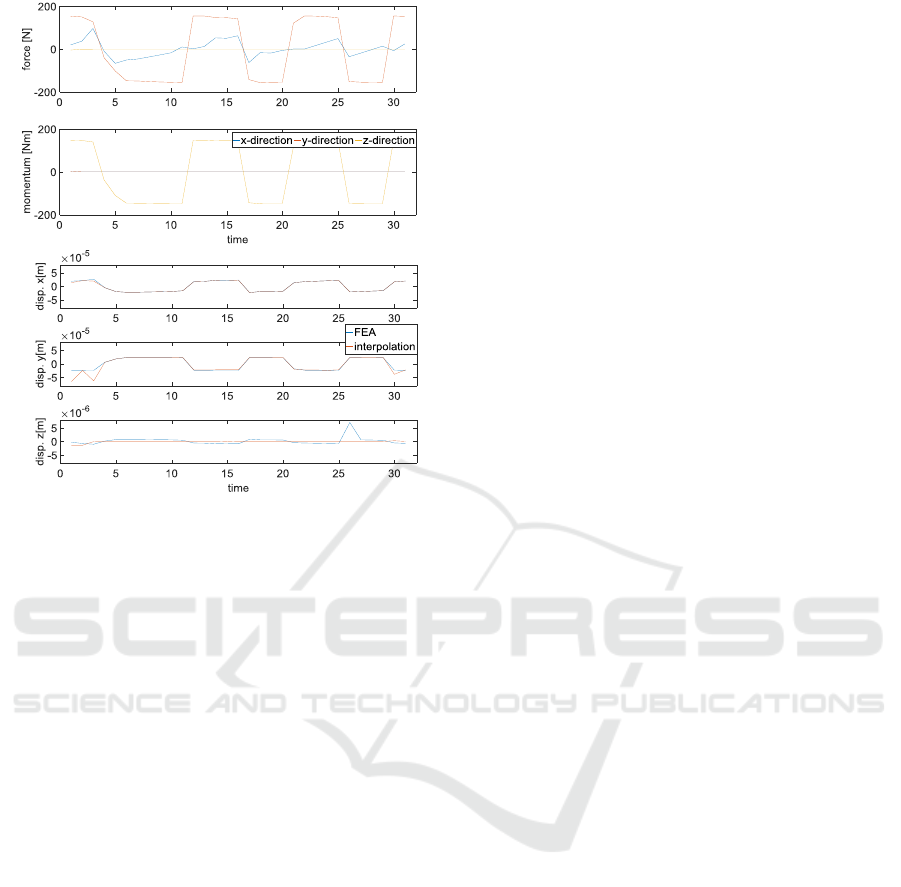
Figure 10: Accuracy of the interpolation method: a) The
same forces and momentums were taken as input for a
FEA and the interpolation method. b) The interpolation
method is able to reproduce the displacements of the FEA.
8 CONCLUSION AND FUTURE
WORK
In this work, a completely new approach for the
interaction between an Overall System Simulation
and structural simulations was developed. Especially
the RBD algorithms of the Overall System
Simulation were vital to perform the task. The
structural simulations were done via FEA.
Unfortunately, both simulation methods have
completely different mathematical and physical
models causing a lack of general acknowledged
approaches to an application-independent, user-
friendly and rather fast interaction.
This work overcomes the difficulties and
completes an existing Virtual Testbed with the
results from structural simulations. This is done by a
bidirectional variable exchange of
forces/momentums and translations/rotations
combined with an interaction. The principle idea of a
variable exchange was followed by other groups as
well. However, this work includes mainly three new
important aspects:
1. The competences of users, algorithms and
models remain separated, which leads to a more
efficient and accurate combined simulation. This is
done by a completely automated interface, that
handles parametrized one-time setup FEA.
2. Structural results are considered in the
dynamic process of the Overall System Simulation,
it is not a static approach.
3. The interaction is implemented in the
framework of an existing Virtual Testbed, which
already represents a powerful tool for Overall
System Simulation for complex models with an easy
to use GUI.
Furthermore, the Virtual Testbed is real-time
capable. The developed interaction saves a huge
amount of time with a one-time setup of a FEA by
an expert and an afterwards automatized structural
simulation. Beyond that, an interpolation method is
introduced and a proof of concept shows, that it is
capable of reproducing structural results. This brings
the completed Virtual Testbed much closer to real-
time capability again than a classical co-simulation
approach. The bidirectional interaction could be
validated with a comparison to an analytical model.
First applications show the new insights that can be
gained with the developed method.
Nevertheless, there is a lot of future work to be
done. First of all, from a technical point of view, the
Delaunay Triangulation should be integrated in C++
code rather than using MATLAB. Another
interesting use case for the interpolation method is
taking results of experiments as lookup-tables
instead of results of performed FEA. In addition, the
lookup-tables could be organized in a library.
For the bidirectional interaction itself, it would
be interesting to give even more power to the end-
user in setting up a desired FEA, e.g. defining
several contact points between Virtual Testbed and
FEA on the same component or import the deformed
component to the Virtual Testbed.
Furthermore, ANSYS Mechanical has a huge
field of different applications not only in structural
simulations, which may allow including other
simulation types, e.g. thermal or fluid, as well.
ACKNOWLEDGEMENTS
This work is part of the project "iBOSS-3",
supported by the German Aerospace Center (DLR)
with funds of the German Federal Ministry of
Economics and Technology (BMWi), support code
50 RA 1504.
a)
b)
Implementing a New Approach for Bidirectional Interaction between a Real-time Capable Overall System Simulation and Structural
Simulations - Completion of the Virtual Testbed with Finite Element Analysis
123

REFERENCES
Bathe, K-J., 1996. Finite Element Procedures. Prentice-
Hall, Inc., New Jersey.
Busch, M., 2012. Zur Effizienten Kopplung von
Simulationsprogrammen. Dissertation in mechanical
engineering at the University Kassel, kassel university
press GmbH, Kassel.
Chung, G-J., Kim, D-H., 2010. Structural Analysis of
600Kgf Heavy Duty Handling Robot. In 2010 IEEE
Conference on Robotics, Automation and
Mechatronics, pp. 40-44.
Dietz, S., Hippmann, G., Schupp, G., 2001. Interaction of
Vehicles and Flexible Tracks by Co-Simulation of
Multibody Vehicle Systems and Finite Element Track
Models. In The Dynamics of Vehicles on Roads and
Tracks, 37, pp. 372-384, Swets & Zeitlinger, 17th
IAVSD Symposium, Denmark.
Hearn, E.J., 1997. Mechanic of Materials 1. Third Edition,
Butterworth-Heinemann, Oxford, Woburn, pp. 299-
300.
Jung, T. J., 2011. Methoden der Mehrkörper-
dynamiksimulation als Grundlage realitätsnaher
Virtueller Welten. Dissertation at RWTH Aachen
University, Departement for Electrical Engineering
and Information Technology.
Kono, D., Lorenzer, Th., Wegener, K., 2010. Comparison
of Rigid Body Mechanics and Finite Element Method
for Machine Tool Evaluation. Eidgenössische
Technische Hochschule Zürich, Institut für Werkzeug-
maschinen und Fertigung.
Michalczyk, K., 2009. Analysis of helical compression
spring support influence on its deformation. In The
Archive of mechanical Engineering, Vol LVI, Number
4, pp. 349-362.
Rieg, F., Steinhilper, R., (Hrsg) 2012. Handbuch
Konstruktion. Carl Hanser Verlag München, Wien, pp.
849-857.
Roßmann, J., Schluse, M., Schlette, C., Waspe, R., 2013.
A New Approach to 3D Simulation Technology as
Enabling Technology for eRobotics. In Van Impe, Jan
F.M and Logist, Filip (Eds.): 1st International
Simulation Tools Conference & Expo 2013,
SIMEX’2013.
Stettinger, G., Benedikt, M., Thek, N., Zehetner, J., 2013.
On the difficulties of real-time co-simulation. In V
International Conference on Computational Methods
for Coupled Problems in Science and Engineering,
Coupled Problems, S. Idelsohn, M. Papadrakakis,
B.Schrefler (Eds.).
Stettinger, G., Horn, M., Benedikt, M., Zehetner, J., 2014.
Model-based Coupling Approach for non-iterative
Real-Time Co-Simulation. Conference paper European
Control Conference (ECC), France.
Stewart, D., Trinkle, J.C., 2000. An Implicit Time-Stepping
Scheme for Rigid Body Dynamics with Coulomb
Friction. ICRA.
Wang, X., Mills, J.K., 2004. A FEM Model for Active
Vibration Control of Flexible Linkages. In
Proceedings of the 2004 IEEE International
Conference on Robotics and Automation, New
Orleans, LA, pp. 4308-4313.
Weise, J., Brieß, K., Adomeit, A., Reimerdes, H.-G.,
Göller, M., Dill-mann, R., 2012. An Intelligent
Building Blocks Concept for On-Orbit-Satellite
Servicing. In Proceedings of the International
Symposium on Artificial Intelligence, Robotics and
Automation in Space (iSAIRAS), Turin (Italy).
Wellmer, G., 2014. Ein partitioniertes Verfahren für die
aeroelastische Freiflugsimulation. Einreichung zum
Deutschen Luft- und Raumfahrtkongress 2014, Docu-
mentID: 340310.
APPENDIX
The spring constant of a compression spring can
be defined in two ways. First, it can be done
experimentally by using the linear relation between
the compression and the force:
(12)
On the other hand, it can be calculated using
certain material criteria and manufacturing
parameters ((Hearn, 1997), see Table 1 for definition
of the variables):
(13)
The rotation of a compression spring is
described and validated in (Michalczyk, 2009).
(14)
In this equation, the total length of the wire
and the slope angle were defined.
(15)
The manufacturing parameters of the spring
modelled for the validation were taken from a usual
SIMULTECH 2017 - 7th International Conference on Simulation and Modeling Methodologies, Technologies and Applications
124
compression spring made out of stainless steel
1.4310.
Table 1: Manufacturing parameters for the spring of the
FEA model.
Wire diameter
Spring diameter
Relevant turns
Spring length
Shear modulus
Poisson ratio
To get the spring constant out of the FEA and the
Overall System Simulation, a linear regression was
used (see Figure 11 and Figure 12).
Figure 11: Linear regression to get the spring constant out
of the FEA model.
Figure 12: Linear regression to get the spring constant out
of the Overall System Simulation.
Implementing a New Approach for Bidirectional Interaction between a Real-time Capable Overall System Simulation and Structural
Simulations - Completion of the Virtual Testbed with Finite Element Analysis
125
