
Sliding Modes based Nonlinear PID Controller for Quadrotor
Theory and Experiment
Yasser Bouzid
1
, Houria Siguerdidjane
2
and Yasmina Bestaoui
1
1
IBISC Laboratoire, Université Paris-Saclay, Evry, France
2
L2S, Centrale Supélec, Université Paris-Saclay, Gif sur yvette, France
Keywords: UAV, Trajectory Tracking, Flight Control, Nonlinear PID.
Abstract: In this paper, a Nonlinear PID (NLPID) control design is proposed. The main idea consists of combining the
classical sliding modes approach together with the PID structure. Unlike the existing nonlinear PID
controllers in the literature, the coefficients are constant parameters in this work. Within this paper, we
investigate the efficiency and the performance of this technique through an application to a small Vertical
Take Off and Landing (VTOL) Unmanned Aerial Vehicle (UAV). The NLPID based autopilot drives the
vehicle toward the desired configuration in the space while stabilizing the roll and the pitch angles where
the closed-loop system stability analysis is highlighted. The numerical simulations have shown satisfactory
results using nominal model or disturbed one compared to the use of classic sliding modes technique only.
Experimental tests are performed to validate the effectiveness of the proposed control approach.
1 INTRODUCTION
Because of their layout topology, the quadrotors are
capable of Vertical Take-Off and Landing (VTOL)
and they have a high maneuverability. In the last
couple of years, they are becoming more popular in
the commercial, academic, and hobbyist sectors. The
challenge that must be addressed by the researchers
is to design flight controllers, insuring good
performance with good level of robustness, knowing
that this is a multi-variable, nonlinear and very
unstable system. This has attracted the interest of
many researchers in aeronautics and robotics (Yang
and Lee, 2014; Bouzid et al., 2016a; Kun and
Hwang, 2016).
The desire to constantly improve the performance
of controlled systems leads to more complexity and
may include strong nonlinearities. As the analysis and
synthesis of control laws used in the linear domain are
often inadequate for nonlinear systems, therefore, a
little sophisticated methods then become necessary to
endeavor (Zou, 2017; Bouzid et al., 2016b).
In this work, we investigate the design of an
efficient control law, robust and readily
implementable, which may provide good performance
for VTOL vehicles in order to classify the robustness
and performance level of different approaches
according to operation conditions in a next
forthcoming work. For this purpose, a Nonlinear PID
(NLPID) control is applied to stabilize the vehicle’s
attitude while the tracking of 3D reference trajectories
is well ensured. This controller is proposed in order to
alleviate the chattering problem of the sliding mode
controllers and allows a direct tuning of the
controller’s parameters that easily allows meeting the
fixed desired specifications with good robustness
level. The properties of this technique will be further
discussed.
The rest of this paper is organized as follows:
Section 2 introduces the mathematical model of the
vehicle. Section 3 presents the synthesis of the so-
called NLPID control. The application of this
technique for quadrotor is described in Section 4
where a stability proof is detailed. In Section 5, the
results obtained from numerical simulations as well
as from the experimental tests, are given under
different operating conditions. Finally, Section 6
contains the conclusion.
2 VEHICLE DYNAMICS
BACKGROUND
The system operates in two coordinate frames: the
inertial fixed frame
(,,,) and the body
286
Bouzid, Y., Siguerdidjane, H. and Bestaoui, Y.
Sliding Modes based Nonlinear PID Controller for Quadrotor - Theory and Experiment.
DOI: 10.5220/0006433402860294
In Proceedings of the 14th International Conference on Informatics in Control, Automation and Robotics (ICINCO 2017) - Volume 1, pages 286-294
ISBN: 978-989-758-263-9
Copyright © 2017 by SCITEPRESS – Science and Technology Publications, Lda. All rights reserved
frame
(
,
,
,
) (Figure 1). Let=
(
,,
)
describes the orientation of the aerial
vehicle (Roll, Pitch, Yaw) and χ=
(
,,
)
denotes
its absolute position with≠±
,≠±
.
We give a brief explanation of the classic process
followed to derive a simplified model that describes
the drone’s in-flight behavior where more accurate
dynamic models may be found as for instance in
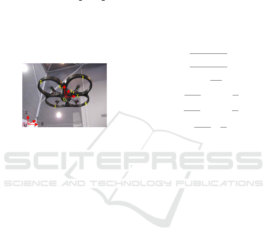
(Kun and Hwang, 2016). The structure and the
propellers are rigid and symmetric (with a suitable
choice of the body reference frame as depicted in
Figure 1, the inertia matrix is diagonal).
Figure 1. Quadrotor in experimentations.
Gravity force that acts on the center of mass is
expressed in the earth fixed frame in the negative
direction. The total thrust is in the positive
direction and expressed in the body fixed frame.
Then, it must be rotated into the earth fixed frame.
The rotation matrix ℛ
(
,,
)
is given by
ℛ=
−
+
+
−
−
where
(.)
and
(.)
are abbreviations for (.) and
(.) respectively. Therefore, the translational
dynamic may be expressed as follows
χ
=−
+
ℛ
(
,,
)
(1)
where
=(0,0,1)
denotes the unit vector of Z-
axis, the mass, the gravity acceleration
and
the total thrust.
Pitch and roll movements, are created by the
difference in combined thrust in the opposite sides
of the vehicle. However, yaw movement is
generated by the differential drag forces. The
rotational dynamics can be expressed as
=−×+
+
(2)
=
,
,
denotes the angular velocity
vector, =(
,
,
) is the diagonal inertia
matrix, =
(
,
,
)
is the control torque and
=
Ω
,
Ω
,0
denotes the propellers
gyroscopic effect with
denotes the rotors inertia
and Ω
is a mixer of the rotors speeds. The angular
velocity of the quadrotor is tranformed into Euler
angular speeds. This yields (Kun and Hwang,
2016)
=
1s
tan c
tan
0c
−s
0s
/c
c
/c
(3)
For real life applications (inspection, coverage,
etc.) or hovering and by using equations (1), (2) and
(3) the simplified dynamic model of the vehicle
may be written as:
χ=
+
−
−+
(4)
=
−
+
Ω
+
(
−
)+
Ω
+
(
−
)+
(5)
3 NONLINEAR PID
CONTROLLER DESIGN
In this paper, an improvement has been brought in
order to simplify the existing controllers, and thus
overcome some issues poorly tackled by the classic
linear or nonlinear techniques, using NLPID.
Usually the kind of control called “NLPID control”
stands for the regulator for which the coefficients are
not assumed to be linear. More precisely, in the
literature, the controllers called nonlinear PID are
those with gains adjusted according to the state or
those with gains depending on the phase (Seraji,
1997). Unlike those mentioned above, our control
law is defined in a novel way. It consists of a
nonlinear controller, which is derived from a method
based upon Sliding Mode Control (SMC) theory and
combined with a PID structure. In Reference (Eker,
2006), a sliding surface that has a PID structure is
used in order to design a sliding mode controller.
This latter is proposed to improve the performance
of the standard sliding mode one. The same idea is
employed later for the steering of lateral moving
strip in hot strip rolling (Choi and Lee, 2009).
Herein, the switching term of the sliding model is
replaced by a PID structure that uses the sliding
surface as an input instead of the tracking error
between the reference and the measured signals.
Sliding Modes based Nonlinear PID Controller for Quadrotor - Theory and Experiment
287

3.1 Controller Design
Consider a class of nonlinear SISO system for ∈
[0,∞) given by:
(
∑
)
=ℱ
(
)
+
(
)
=ℎ
(
)
(6)
where ∈ℝ
is an -dimentional state vector, ∈
ℝ is a scalar input, ∈
⊂ℝ
is a scalar output,
ℱ:
⇢ℝ
and :
⇢ℝ
are -dimentional
vector functions sufficiently smooth on a domain
⊂ℝ
and ℎ() the output scalar function.
Assumption (A1): There exists a diffeomorphism
:
⇢
where
=(
) is a domain that
contains the origin and a change of variables =
() that transforms the nonlinear system into an
equivalent system given by
∑
(
)
=
(
)
(
)
=
(
)
+
(
)
=
(7)
=1…−1.
(
)
,
(
)
denote continuous
nonlinear functions and
(
)
is nonsingular for all
∈
.
Now, let us consider a general sliding surface
form
(
)=
+
(t)
(8)
where
=−
represents the tracking error
between a reference trajectory
and the output
and
a positive constant.
By expansion, equation (8) may be written as
=
(
)
(
)
+
∑
(
)
(
)
(9)
where
,=0,…,−2 are positive tuning
parameters provided that they are chosen in order to
render the equilibrium,
=0, asymptotically
stable in finite time T.
The first-order time derivative of
is
=
(
)
(
)
+
∑
(
)
(10)
Using the last component of system (7), where
Assumption (A1) holds, equation (10) becomes
=
(
)
+
(
)
−
(
)
(
)
+
∑
(
)
(11)
Given a positive definite Lyapunov function
candidate
=
1
2
(12)
The first-order time derivative of leads to
=
(13)
Note that the reachability condition of sliding
mode control ensures the asymptotic stability (
<
0). Thus,
is forced to satisfy the following
inequalities
<0ℎ
>0
>0ℎ
<0
(14)
Assuming that
=−
(
)
(15)
with being a strictly positive constant and
(
)
is a
function defined by
(
)
<0<0
(
)
=0=0
(
)
>0>0
(16)
we ensure inequalities (14). In fact,
(
)
may take
different forms of sigmoid. The discontinuous
function
(
)
=
(
)
, represents the ideal sliding
modes regime.
From (11) and (15), it immediately follows that
=
(
)
{
(
)
+
∑
(
)
−
(
)
(
)
+
(
)
}
(17)
The discontinuous term
(
)
allows a good level
of robustness with respect to uncertainties and
disturbances. However, the fast oscillation of the
control signal (chattering phenomena), gives rise of
vibration in the system during the flight where these
dynamics are not sustained by the rotors. So, in
order to improve the performance of the controller
limiting the effect of the chattering phenomena,
involved through the term
, and meet readily
the specification of the control, we combine a PID
structure and controller (17) determined above.
=
(
)
{+
∑
(
)
−
(
)
(
)
+
(
)
}
(18)
When the state trajectory lies on the sliding
surface i.e.,
(
)
= 0, the design problem of the
sliding surfaces can be regarded as a linear state
feedback equivalent control design. Therefore, from
(17) and (18), the equivalent control is found by
recognizing that
(
)
= 0. This is a necessary
condition for the state trajectory to lie on the sliding
surface. As known, the switching term holds when
the trajectories are not on the sliding surface in order
to bring these trajectories to this surface. Therefore,
we proceed by using this surface as an input of the
PID structure to ensure that
(
)
converges toward
the origin (
(
)
→0) and then we ensure the
convergence of the trajectories toward this surface.
Therefore, the controller may be written as
=
(
)
(
)
+
(
)
+
(
)
+
∑
(
)
−
(
)
(
)
+
(
)
(19)
,
and
denote the proportional gain, the
derivative and integral time constants respectively.
ICINCO 2017 - 14th International Conference on Informatics in Control, Automation and Robotics
288

This new approach is clarified by Figure 2.
Figure 2: Nonlinear PID control architecture.
3.2 Some Properties of the Proposed
Controller
The proposed technique builds on the SMC
paradigm and uses a dynamic inversion-like control
strategy to linearize the system. Unlike the SMC
strategy, obtained controller (19) guarantees that the
tracking error of the closed loop nominal linearized
system goes to the origin by forcing the tracking of
the sliding surface (namely
=0) via the PID
controller. The absence of actual sliding action in the
proposed technique requires a proper stability
theorem (see Section 4.2).
NLPID exhibits several benefits, and can be split
up into two parts: The first part is involved as
dynamic inversion technique in order to compensate
the nonlinearities of the system. This part is
represented by red colored blocks in Figure 2. The
remaining part includes the PID structure, which
represents the additional control needed to guarantee
that the tracking error goes toward the origin by
forcing the tracking of the sliding surface. We can
observe in Figure 2 that sliding surface (9) is the
input of the PID block instead of the tracking error
as the classic one. Of course, this structure is
suggested to keep almost a good level of robustness
even with the absence of the discontinious term that
ensures higher level of robustness.
We observe the absence of discontinuities
associated to jumps in the control action, which
clearly eliminates the chattering problem and
reduces the consumed energy. In addition, the steady
state errors are cancelled by adding the integral
action that penalizes the deviations between the
output and its set point. Therefore, the control
accuracy is improved. Furthermore, this proposed
controller allows meeting quite readily the desired
specification by adjusting the PID parameters on the
hovering conditions. However, the derivative term
of the proposed controller induces a higher order
derivative one with respect to that needed for
classical “Feedback Linearization”. Unfortunately,
this is a drawback because of the additional noise
and derivative estimation inaccuracy. These
properties are shown in Section 5 through a series of
numerical simulations.
4 QUADROTOR APPLICATION
This novel technique is herein applied to the
quadrotor (Multi-input Multi-output system) by
taking care of having an adequate control structure.
In the position control, and are controlled
through two virtual inputs (
,
) that push the
system to reach the prescribed references
and
respectively and allow to generate the reference
angles (
,
) via equation (23). The Euler angles
are controlled by the torque vector
(
,
,
)
,
whereas the altitude is controlled by
. This control
structure allows the vehicle to ensure the tracking of
prescribed trajectories along the three axes (X, Y
and Z) and the yaw angle. We calculate these control
laws by using the NLPID approach as described in
Section 3 where the tracking errors are defined as:
=−
,
=−
,
=−
,
=−
,
=−
and
=−
.
4.1 Autopilot Design
Translation dynamics (4) can be divided into three
other sub-systems along the three axis (X, Y, Z).
Each sub-system has one input (
,
,
and one
output (,,) respectively. We first start with
for the altitude motion. Once this command is
calculated we then proceed in the same way with
and
by considering
as time varying parameter,
with
=c
s
c
+s
s
=s
s
c
−c
s
(20)
Thus, the sliding surfaces are set to:
=
+
|
,,
(21)
where
,
and
are positive constants.
Applying (19), we obtain
=
(
)
+
(
)
.+
(
)
+
−−
=
(
)
+
(
)
.+
(
)
+
−
=
(
)
+
(
)
.+
(
)
+
−
(22)
Sliding Modes based Nonlinear PID Controller for Quadrotor - Theory and Experiment
289

Then, from system (20), the required reference
angles of the roll and pitch rotations are given by
=
−
=
+
(23)
Similarly, system (5) can be divided into three
sub-systems for the roll, pitch and yaw rotations.
Each one of them has one input (
,
,
) and one
output (,,) respectively. Consequently, the
surfaces are
=
+
=
+
=
+
(24)
where (
,
,
) are positive constants.
Finally, the control laws are given by
=−
(
)
+
(
)
.+
(
)
+
+
Ω
+
−
=−
(
)
+
(
)
.+
(
)
+
+
Ω
+
−
=−
(
)
+
(
)
.+
(
)
+
+
−
(25)
Also
(.),
,
(.)
,
(.)
denote the proportional
gain, the integral and derivative time constants of the
NLPID structure respectively.
4.2 Stability Analysis
For the sake of completeness, we study the stability
of the closed loop system using our proposed
approach.
Remark 1: all the sub-systems that describe the
drone’s behavior in flight (three translations and
three rotations), may be considered as two-
dimensional class of systems:
For ∈[0,∞)
=
=
(
χ,
)
+
(
χ,
)
=
(26)
where(
,
)
∈
⊂ℝ
is a 2-dimentional state
vector, ∈ℝ is a scalar input, ∈ℝ is a scalar
output.
For =2, substituting surface expression (9)
into control law (19), the closed loop of system (26)
written in terms of the tracking error vector
components,
=
,
=
(
−
,−
)
is
=
=−
−
+
,
(27)
where:
=
+
+
1+
=
+
1+
,=
1+
(
)
Consider that system (27) can be divided into
nominal system
=
(28)
and an additional integral term,Δ
,∈
×
[
0,∞
)
⊂ℝ
⇢ℝ
, which equals to
Δ
,=
0
,
Thus
=
+Δ
, (29)
where :
⇢ℝ
is a 2-dimentional vector
functions sufficiently smooth on a domain
⊂
ℝ
.
Assuming that the origin of the nominal system
is exponentially stable equilibrium and accepting
that we have established this stability as following:
Let V a Lyapunov function that satisfies:
≤≤
(30)
The first-order time derivative along (28) is
≤−
(31)
and
‖
‖
≤
(32)
for all
∈
and
>0,=1,…,4 where
denotes the gradient operator.
We suppose that
,, in a bounded
neighborhood of the origin, satisfies the following
condition
Δ
,≤
(33)
for all (,
)∈
[
0,∞
)
×
and
>0.
Now, let us use V as a candidate Lyapunov
function to prove the exponential stability of overall
system (29). The first-order time derivative of V
along (29) gives
=
+
Δ
, (34)
Using (31), we get
≤−
+
‖
‖
Δ
,
Inequalities (32) and (33) lead to
≤−
+
(35)
To ensure that the origin of (29) is exponentially
stable equilibrium, the following condition must be
satisfied
ICINCO 2017 - 14th International Conference on Informatics in Control, Automation and Robotics
290
≤
(36)
We summarize this result by Theorem 1.
Theorem 1: Assuming that the origin of system
(28)
is exponentially stable. Let a Lyapunov
function,:
⇢ℝ
, defined for system
(28)
where
(30)
-
(32)
hold in domain
.Assuming that
the integral term
, satisfies inequality
(33)
, if
condition
(36)
is satisfied, then the origin of system
(29)
is also exponentially stable.
This result is only qualitative because the above
proof is done without explicit knowledge of the
Lyapunov function. In the following, we seek to find
a candidate Lyapunov function and the adequate
parameters,
,=1,…,5, which verify equations
(30)-(32). We propose a quadratic candidate
function as
=
(37)
where
=
is a symmetric positive definite matrix. The first-
order time derivative along (28) gives
(
)
=−
+
(
−
)
+
(
−
−
)
(38)
Chosen σ
=1 (see inequality (31)), equation
(38) leads to:
=
+
=
=
(39)
Obviously, the obtained matrix has two
eigenvalues:
,
=
+
∓
√
(40)
where
=
+
+
+
+1
−4
−
1
+
+
+
+1
We have also
=
Then, computing
‖
‖
we obtain
‖
‖
≤
‖
‖
≤
√
2.
(
)
where
(
)
is the maximal value of
eigenvalues
and
of matrix . From (32), it
comes that
=
√
2.
(
)
. Then, closed loop
system (29) is exponentially stable if
≤1/
√
2.
(
)
Theorem 2: Let a quadratic Lyapunov function (37),
for nominal system (28) on domain
, where is
given by (39). If the
,of (29) satisfies
inequality (33) with
≤1/
√
2.
(
)
, then the
origin of system (29) is exponentially stable.
5 SIMULATION STEP AND
EXPERIMENTAL RESULTS
5.1 Numerical Simulations
Numerical simulations have been performed with
the available UAV nominal parameters (Table 1).
Table 1: Quadrotor parameters.
()
0.429
(.
)
.
(.
)
0.0022
(.
) 0.0048
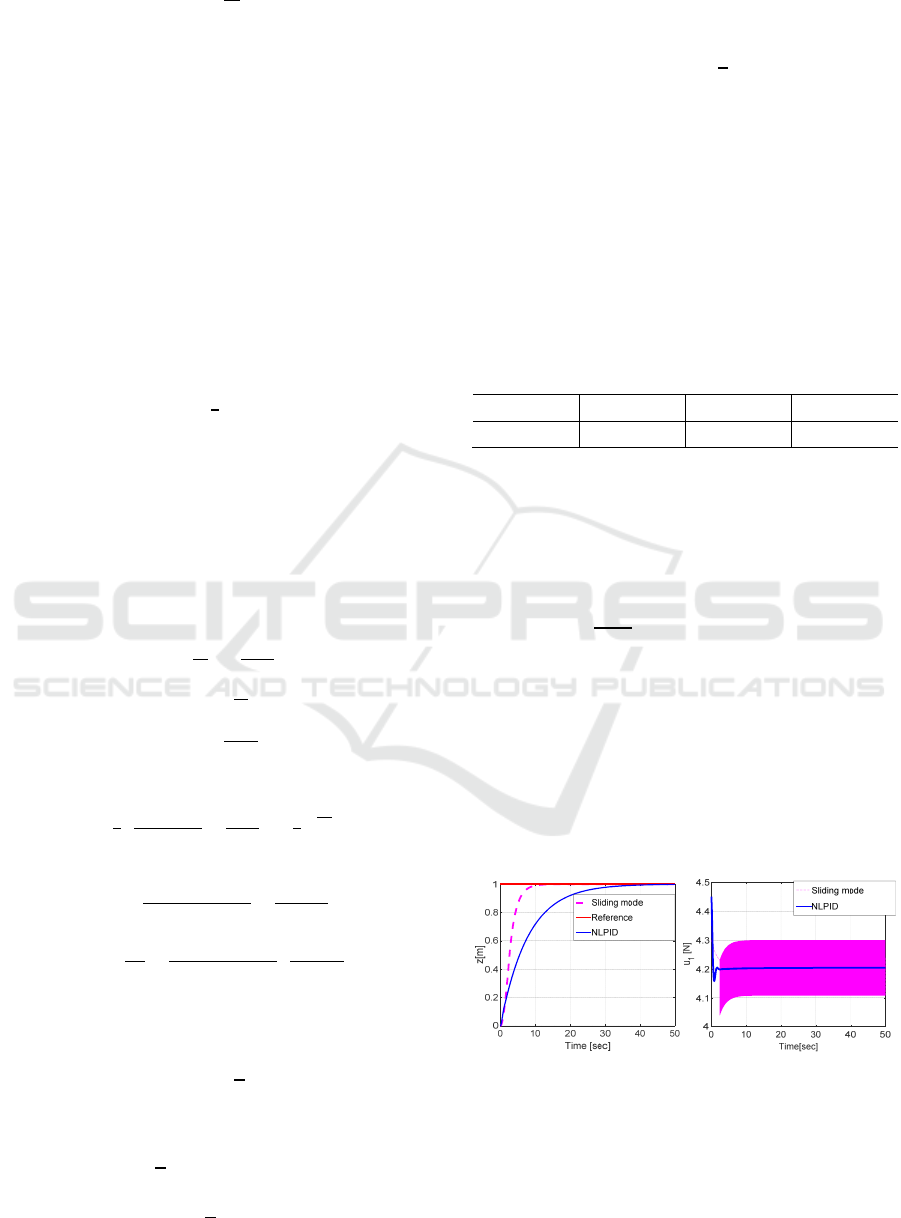
The proposed controller performance is being
compared with the sliding mode controller. For this
purpose, we consider a vertical flight at altitude of
one meter during 50 seconds. The control
parameters are tuned by minimizing the following
objective function using Genetic Algorithms (GA):
=
(
+
()
)
This is in order to obtain a good trade-off between
the faster time response and the consumed energy
where
and
are the final and the initial times
respectively, () is the tracking errors vector and
is the inputs vector. The obtained control parameters
for vertical flight are:
=4.289,
=
18.527,
=0.001 and
=0.126for NLPID
controller;
=21.19 and
=5.18for SMC.
The resulting behaviors are depicted in Figure 3.
Figure 3: Comparison in vertical flight.
From Figure 3, we observe that the NLPID has a
slower time response. However, the command signal
is obviously improved and presents the best control
behavior, which is smoothly varying without
chattering. This kind of control signals is more
adequate for the actuators and allows performing a
Sliding Modes based Nonlinear PID Controller for Quadrotor - Theory and Experiment
291
good control without vibration and with less energy.
Note also that the nonlinear PID exhibits no
overshoot. This is very important benefit because the
overshoot of any time response creates oscillations
of the vehicle during the passage from waypoint to
another one. Moreover, the proposed controller
achieves minor steady state error. This is due to the
inclusion of an integral action term. The additional
parameters are depicted in Table 2.
Table 2: Control parameters comparison.
Control parameters
Vertical motion
Longitudinal
motion
Lateral
motion
Yaw
rotation
NLPID
=4.29
=18.6
=0.01
=0.12
=4.72
=12.43
=0.97
=9.42
=0.63
=1.073
=0.043
=0.56
=4.29
=9.90
=0.9
=10.3
=0.51
=0.04
=0.70
=0.53
=10.8
=11.4
=0.9
=13.9
SMC
=21.19
=5.18
=29.50
=5.18
=1.38
=5.26
=30.92
=6.03
=0.22
=4.05
=31.6
=5.1
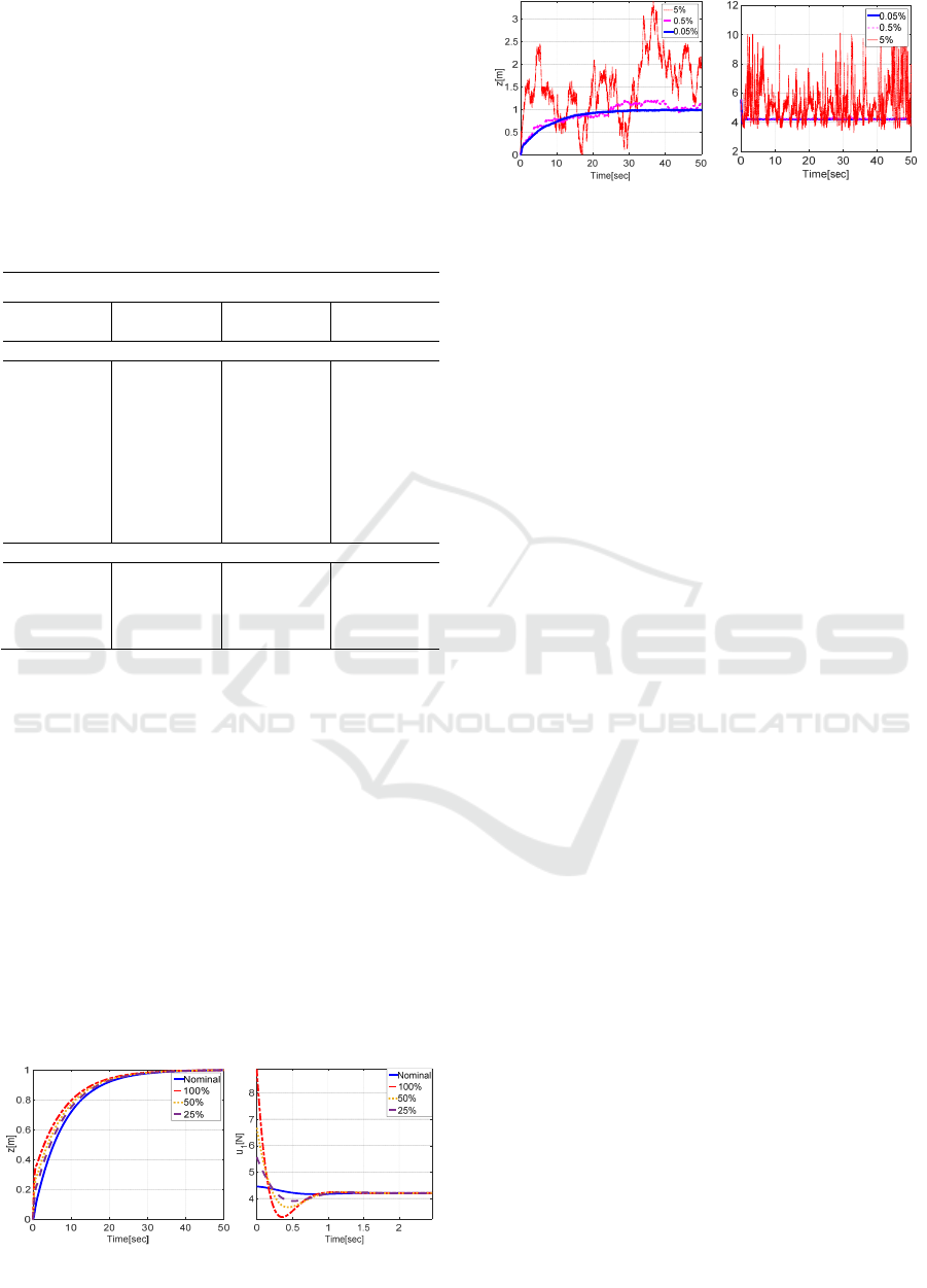
Now, let us check the effectiveness of the control
laws and their level of robustness. Firstly, we
consider uncertainties of 25%, 50% and 100% in the
parameters with respect to the nominal values given
in Table 1. Then, we suppose an additive Gaussian
noise affecting the measured signals with different
magnitudes of 5%, 0.5% and 0.05% respectively.
The obtained results are shown in Figure 4 and
Figure 5.
It should be noted from Figure 4 that the
quadrotor motors generate an additional thrust at the
start up in order to ensure the desired control.
Furthermore, in this case of model parameters
uncertainties, the controller is able to, accurately;
ensure the tracking of the desired set point. Figure 5
illustrates that the high noise magnitude reduces the
Figure 4: Comparison for parameters uncertainties
scenario.
Figure 5: Comparison considering noisy measurements.
performance of the controller only, which still
ensures the stability of the system.
The advantage of this novel controller is: its low
sensitivity to the model uncertainties while adequate
control signals are delivered.
Now, let’s check the effectiveness of the
controller in the case of time varying reference
trajectory. For this particular example, the UAV has
to stabilize its attitude while following a helix
trajectory, having radius of 10 meters. The
simulation-compared results are sketched in Figure
6.
Figure 6 shows the stable tracking behavior of
the complete closed loop system where the outputs
converge to the desired trajectory with minor steady
state errors.
5.2 Experimental Results
To validate the proposed autopilot through a series
of experimental tests, we have used an available X-
shaped quadrotor aerial platform (AR-drone V2).
The designed autopilot was implemented in C++
under Robot Operating System (ROS) open source
framework using a publisher/subscriber paradigm
that ensures all communications between real robots
(for more details see: ros.org). The position in the
plan XY is determined using the frontal camera
based on Parallel Tracking and Mapping (PTAM)
algorithm developed in (Engel et al., 2012). The
main program runs on the ground station, which
communicate with the quadrotor via Wi-Fi link.
In this simple proposed scenario, the desired
trajectory is formed by successive straight-line
segments. The vehicle starts from the origin to reach
the point
(
,,
)
=(2,2,1).
In Figure 7, we observe that the outputs converge
to the desired trajectory with significant steady state
accuracy. The control signals seem to be in
acceptable form where the magnitudes stay within
the allowable ranges (see Figure 8). Overall, this
experimental test confirms the simulation results and
shows the effectiveness of the technique.
u
1
[N]
ICINCO 2017 - 14th International Conference on Informatics in Control, Automation and Robotics
292
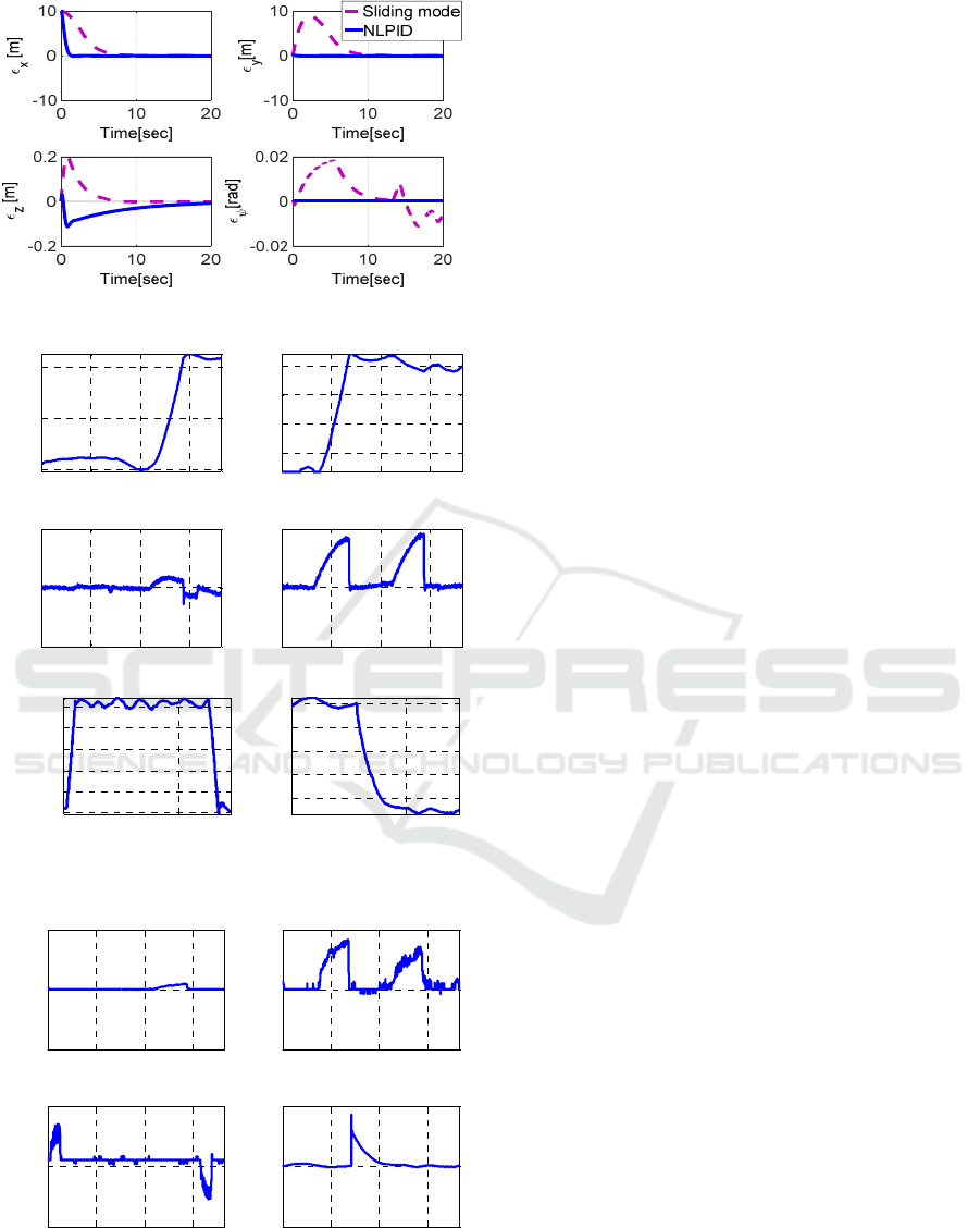
Figure 6: Tracking errors time responses.
Figure 7: System time responses.
Figure 8: Control signals.
6 CONCLUSIONS
A quadrotor model was simplified in order to
elaborate simple control laws for a purpose of
implementation. A novel control design was
proposed. It is shown that this method guarantees
exponential stability. Numerical simulations were
carried out in order to evaluate the effectiveness of
the designed control system. Besides, experimental
tests were performed. One may guess that, as matter
of fact, the proposed methodology turns out to take
profit of the advantages that may be brought by the
PID and SMC controllers simultaneously and left
aside their eventual drawbacks. In addition, the
robustness against model uncertainties by choosing
appropriate control parameters are guaranteed. Due
to the fact that the use of sign function in the sliding
mode control leads to high oscillations in the control
signals, which is undesired chattering phenomenon,
so, we introduced a nonstandard PID structure as a
possible solution to overcome this drawback whilst
the steady state errors vanishes under the effect of
the integral action. In the near future work, we will
study the stability of the system considering
saturation modules to imitate the real case.
REFERENCES
Bouzid, Y., Siguerdidjane, H., Bestaoui, Y., Zareb, M.,
2016a. Energy Based 3D Autopilot for VTOL UAV
Under Guidance & Navigation Constraints. J. Intell.
Robot. Syst. 1–22. doi: 10.1007/s10846-016-0441-1.
Bouzid, Y., Siguerdidjane, H., Bestaoui, Y., 2016b.
Improved 3D trajectory tracking by Nonlinear Internal
Model-Feedback linearization control strategy for
autonomous systems. IFAC-Pap., 6th IFAC
Symposium on System Structure and Control SSSC
2016Istanbul, Turkey, 22—24 June 2016 49, 13–18.
doi:10.1016/j.ifacol.2016.07.480.
Choi, Y.-J., Lee, M.C., 2009. PID sliding mode control for
steering of lateral moving strip in hot strip rolling. Int.
J. Control Autom. Syst. 7, 399–407. doi:10.1007/
s12555-009-0309-2.
Eker, İ., 2006. Sliding mode control with PID sliding
surface and experimental application to an
electromechanical plant. ISA Trans. 45, 109–118.
doi:10.1016/S0019-0578(07)60070-6.
Engel, J., Sturm, J., Cremers, D., 2012. Accurate Figure
Flying with a Quadrocopter Using Onboard Visual and
Inertial Sensing, in: In Proc. of the Workshop on
Visual Control of Mobile Robots (ViCoMoR) at the
IEEE/RJS International Conference on Intelligent
Robot Systems (IROS).
Kun, D.W., Hwang, I., 2016. Linear Matrix Inequality-
Based Nonlinear Adaptive Robust Control of
0 20 40 60
0
1
2
x[m]
Time[sec]
0 20 40 60
0.5
1
1.5
2
y[m]
Time[sec]
0 20 40 60
-5
0
5
φ
[°]
Time[sec]
0 20 40 60
-5
0
5
θ
[°]
Time[sec]
0 50
-0.2
0
0.2
0.4
0.6
0.8
z[m]
Time[sec]
0 50
0
20
40
60
80
ψ
[°]
Time[sec]
0 20 40 60
-1
0
1
u
2
[N.m]
Time[sec]
0 20 40 60
-1
0
1
u
3
[N.m]
Time[sec]
0 20 40 60
2
4
6
u
1
[N]
Time[sec]
0 20 40 60
-1
0
1
u
4
[N.m]
Time[sec]
Sliding Modes based Nonlinear PID Controller for Quadrotor - Theory and Experiment
293

Quadrotor. J. Guid. Control Dyn. 39, 996–1008.
doi:10.2514/1.G001439.
Seraji, H., 1997. A New Class of Nonlinear PID
Controllers for Robotic Applications.
Yang, H., Lee, D., 2014. Dynamics and control of
quadrotor with robotic manipulator, in: 2014 IEEE
International Conference on Robotics and Automation
(ICRA). Presented at the 2014 IEEE International
Conference on Robotics and Automation (ICRA), pp.
5544–5549. doi:10.1109/ICRA.2014.6907674.
Zou, Y., 2017. Nonlinear robust adaptive hierarchical
sliding mode control approach for quadrotors. Int. J.
Robust Nonlinear Control 27, 925–941. doi:10.1002/
rnc.3607.
ICINCO 2017 - 14th International Conference on Informatics in Control, Automation and Robotics
294
