Path Planning and Obstacles Avoidance using Switching Potential
Functions
Giuseppe Fedele
1
, Luigi D’Alfonso
2
, Francesco Chiaravalloti
3
and Gaetano D’Aquila
2
1
Department of Informatics, Modeling, Electronics and Systems Engineering, University of Calabria,
Via Pietro Bucci, 42C, 87036, Rende, Italy
2
GiPStech s.r.l, 87036, Rende, Italy
3
IRPI - CNR, 87036, Rende, Italy
Keywords:
Mobile Robots Path Planning, Obstacles Avoidance, Artificial Potentials Field Method.
Abstract:
In this paper, a novel path planning and obstacles avoidance method for a mobile robot is proposed. This
method makes use of a switching strategy between the attractive potential of the target and a new helicoidal
potential field which allows to bypass an obstacle by driving the robot around it. The new technique aims at
overcoming the local minima problems of the well known artificial potentials method, caused by the summa-
tion of two (or more) potential fields. In fact, in the proposed approach, only a single potential is used at a
time. The resulting proposed technique uses only local information and ensures high robustness, in terms of
achieved performance and computational complexity, w.r.t. the number of obstacles. Numerical simulations
and comparisons with traditional artificial potential field technique confirm a robust behavior of the method,
also in the case of a framework with multiple obstacles.
1 INTRODUCTION
Robot motion planning and obstacles avoidance have
been a research topic for around three decades. The
problem can be formulated as follows: given an ini-
tial position of the robot, it should compute how to
gradually move itself to the desired goal placement,
without entering in the obstacles regions.
When an exhaustive knowledge about the envi-
ronment and all the obstacles inside, is available, the
robot path planning can be performed offline before
the execution starts. Methods based on these assump-
tions belong to the family of global path planning
techniques. The global path planning problem is well
studied and fairly solved (see(Mac et al., 2016)). Tra-
ditional techniques are cell decomposition method,
shown by (Rosell and Iniguez, 2005;
ˇ
Seda, 2007),
and roadmap based techniques, described by (Choset
et al., 2005) and (Bopardikar et al., 2015). Other ap-
proaches are based on set-theoretic arguments cou-
pled with a receding horizon control algorithm and
have been proposed by (Franz
`
e and Lucia, 2015).
However, in a real context, the environment is usu-
ally partially known and having a complete knowl-
edge of the obstacles and their positions in advance
is unrealistic. In this case, information from available
sensors has to be continuously updated resulting in a
more complex planning problem. This situation is de-
noted as online path planning or local path planning
and it has been described by (Chu et al., 2012). In
this context, some of the solutions have been formu-
lated by applying traditional approaches to real-time
motion planning, e.g. (Lau et al., 2013), (Chamber-
land et al., 2010). In order to avoid the inefficiency
of traditional methods, research interest is pointing to
new approaches based on neural networks ((Yang and
Meng, 2000)), fuzzy logic ((Araujo, 2006)) and na-
ture inspired methods like genetic algorithms ((Ala-
jlan et al., 2013)). Other approaches face the prob-
lem using one-step ahead controllable sets and ro-
bust positively invariant regions, see (Franz
`
e and Lu-
cia, 2016), and mathematical approaches ((Benzer-
rouk et al., 2012), (Kim and Kim, 2003)). In par-
ticular, the latter papers face the obstacles avoidance
problem by adapting limit cycles theory to the context
of interest. If an obstacle has to be bypassed, an ar-
tificial limit cycle is placed on it and is used to drive
the robot around it.
Both local and global algorithms have advantages
and drawbacks. Global planning allows for optimal
paths design but these methods are not robust to avoid
moving obstacles when high computational power is
Fedele, G., D’Alfonso, L., Chiaravalloti, F. and D’Aquila, G.
Path Planning and Obstacles Avoidance using Switching Potential Functions.
DOI: 10.5220/0006427703430350
In Proceedings of the 14th International Conference on Informatics in Control, Automation and Robotics (ICINCO 2017) - Volume 2, pages 343-350
ISBN: Not Available
Copyright © 2017 by SCITEPRESS – Science and Technology Publications, Lda. All rights reserved
343

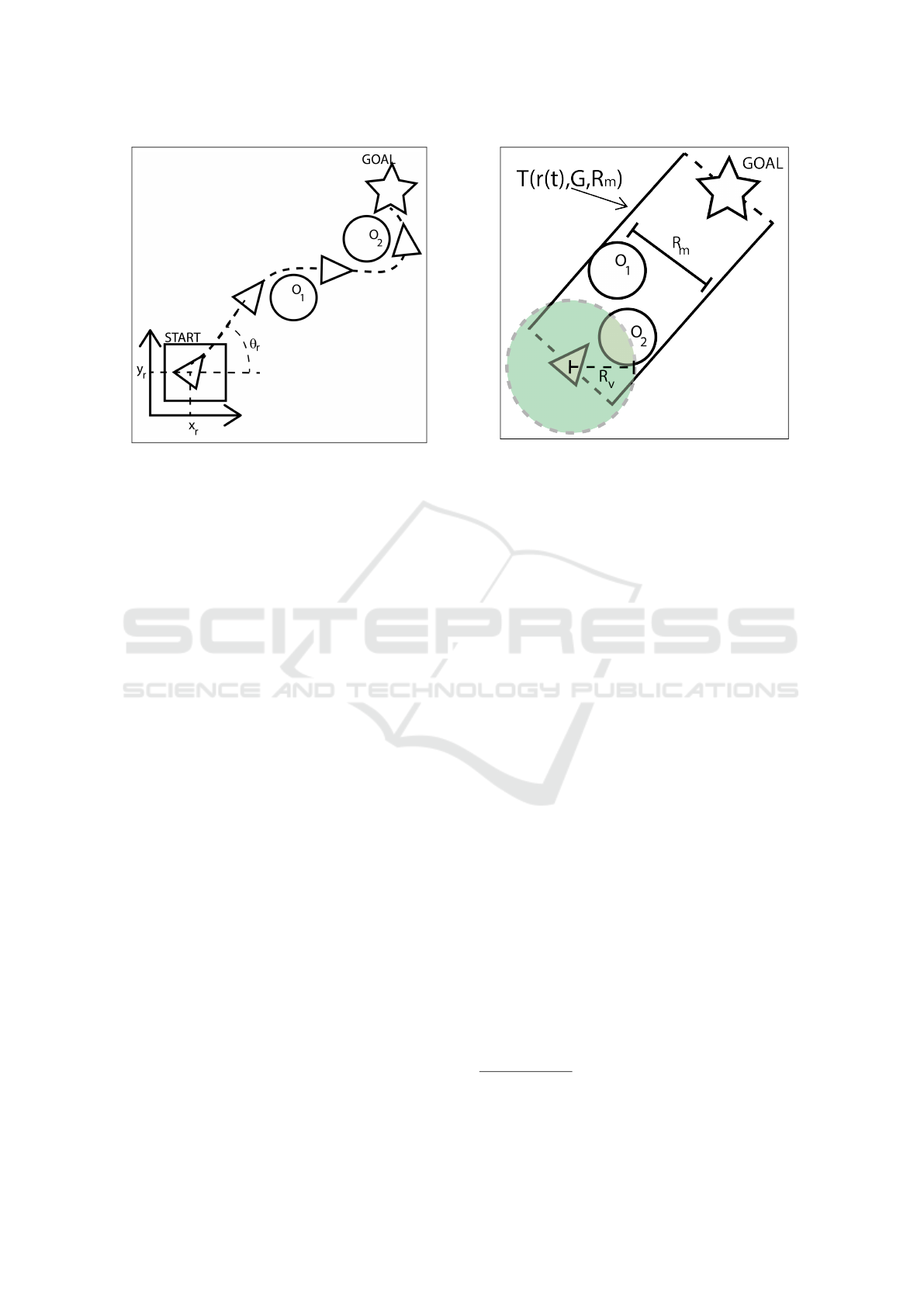
Figure 1: Configuration example.
not available. On the other hand, local path planning
methods can be used also in the case the obstacles
are not static but their performance are really affected
by robot sensors quality and robot allowed maximum
velocity. Moreover, in a local point of view, global
optimality criteria usually cannot be satisfied.
Aiming at enhancing both methods advantages,
avoiding their drawbacks, some techniques based on
the combination of local and global path planning
have been developed by (Zhang et al., 2012) and (Bi
et al., 2008).
The artificial potentials method (APF) is one of
the first solutions proposed to solve the planning prob-
lem online. The basic concept of APF has been pre-
sented in the seminal work by (Khatib, 1990) where
the author proposes to fill the robot’s workspace with
an artificial potential field in which the robot is at-
tracted to its goal position and is repulsed away from
the obstacles. To this end a potential function which
sums the effects of both attractive and repulsive po-
tentials is used. However, as stated by (Siciliano et al.,
2008), the summation of a repulsive potential field
and of an attractive one may result in local minima,
when the repulsive potential is equal to the attractive
one in the same area.
In this paper, a novel approach to the artificial po-
tentials field method is described. To avoid local min-
ima problems due to the superposition of two or more
potentials, the proposed method uses only one artifi-
cial potential field at a time, choosing it between an
attractive one or an obstacle bypassing one. The po-
tential field selection is performed following a set of
rules with no requirements about global information
on the positions of all the obstacles. Moreover, a new
potential field is proposed which allows to bypass an
obstacle by going around it. Since only local informa-
Figure 2: Detection field and T (r(t),G,R
m
) region: O
2
sat-
isfies Eq. (7).
tion is used, the proposed technique ensures high ro-
bustness, in terms of achieved performance and com-
putational complexity, w.r.t. the number of obstacles.
The paper is organized as follows: in Section 2 the
problem is stated; in Section 3 the proposed helicoidal
potential field is described; in Section 4 the path plan-
ning and obstacles avoidance rules are shown; a new
Lyapunov based control law is proposed in Section 5;
in Section 6 numerical results are shown and the last
Section is devoted to conclusions.
2 PROBLEM STATEMENT
Let r(t) = [x
r
(t),y
r
(t),θ
r
(t)]
T
be the pose (position
and orientation) of a moving robot and let {O
i
=
[x
O,i
,y
O,i
]
T
},i = 1,.. .,N be a set of circle shape static
fat obstacles, with center in [x
O,i
,y
O,i
]
T
and known ra-
dius R
i
, computed considering the robot size
1
. The fat
obstacles are assumed to not intersect so that the robot
is always allowed to go between two obstacles. Note
that there is no loss of generality due to this assump-
tion since if two obstacles are near enough to have an
intersection between their fat versions, then a single
bigger fat obstacle can be considered which circum-
scribes them. Fig. 1 depicts a possible configuration
of the robot and the obstacles.
The robot is assumed to have a detection field of
R
v
meters and to be able of inferring each obstacle
in the detection field. Two kinds of detection may
occur: in the first case, the center of the obstacle is
1
If the obstacle shape is not circle-like, than the circum-
scribing circle can be considered instead of real obstacle
shape.
ICINCO 2017 - 14th International Conference on Informatics in Control, Automation and Robotics
344

inside the detection field, in the second one, only a
portion of the obstacle is detected. In the latter case,
a virtual obstacle can be considered instead of the one
detected, placing it in the nearest portion of the obsta-
cle detected by the robot and assuming that the virtual
radius is equal to the actual distance from the robot to
the detected obstacle portion. For the sake of sim-
plicity, in the following the results will be described
assuming that the centers of all the obstacles into the
detection field are available.
Note that this is not a restrictive assumption since
it can be easily accomplished by equipping the robot
with distance or vision based sensors. Fig.2 shows an
example of obstacle detection field.
Moreover the robot is assumed to have knowledge
about its current pose and about the goal position, de-
noted as G = [x
G
,y
G
]
T
. To this end, depending on
the environment configuration, GPS based localiza-
tion techniques (outdoor configurations) or SLAM al-
gorithms (indoor configurations) may be used to pro-
vide the required information to the robot.
This work aims at planning a feasible path for
the mobile robot so that the desired goal position
G is reached avoiding collisions with the obstacles
{O
i
},i = 1,.. .,N.
3 OBSTACLE BYPASSING
POTENTIAL
The artificial potentials path planning method relies
on the use of artificial potential fields to simultane-
ously reach the desired position avoiding obstacles in
the robot environment. The goal is assumed to gen-
erate an attractive potential field U
a
(r(t),G) and each
obstacle O
j
is assumed to generate a repulsive poten-
tial field U
r
(r(t),O
j
). The robot moves in the con-
figuration space under the influence of the artificial
potential field
U
sum
(t) = U
a
(r(t),G) +
N
∑
j=1
U
r
(r(t),O
j
) (1)
which has to drive the robot to the goal, using the
attractive part, and simultaneously repel the robot
from the obstacles. At this point, planning is per-
formed in an incremental way. The negative gradi-
ent −∇U
sum
(r(t)), representing the most promising
direction of local motion to reach the goal, is used
at each robot configuration r(t), to obtain the robot
command input.
Despite its simplicity, the artificial potentials
method, in its traditional formulation, is affected by
known local minima problems, as shown by (Park and
Lee, 2003).
In the traditional artificial potentials method, the
bypassing of an obstacle is provided by summing an
attractive and a repulsive potential. If only the repul-
sive potential is used, the robot is taken away from the
obstacle but it is not driven to the goal and no assur-
ance about moving in a pose where the obstacle can
be bypassed is given. In this context, a new artificial
potential is now proposed, the main idea of which is
to allow for bypassing an obstacle by going around it
using the effects of only one artificial potential.
Figure 3: Helicoid (2) centered in (x
0
,y
0
) = (1,1) with c =
1/3, 0 ≤ r ≤ 1 and 0 ≤ ζ ≤ 5.
A useful configuration to avoid an obstacle con-
sists in having field lines of the gradient that turn
around the obstacle. In particular, in the case of a cir-
cular obstacle, in the sense defined above, a suitable
geometry is obtained with closed-like circular field
lines centered in the position of the obstacle.
This configuration can be obtained starting by
the circular helicoid described in parametric form by
(Struik, 1961):



x = x
0
+ r cos(ζ)
y = y
0
+ r sin(ζ)
z = cζ
(2)
which represents the minimal surface in R
3
having
a circular helix of radius r and centered in x
0
,y
0
, as its
boundary (Fig. 3).
The parameter ζ determines the number of wind-
ings of the surface. For example, if 0 ≤ ζ ≤ 2π there
is a single full-twist.
In Cartesian coordinates Eq. (2) becomes:
y − y
0
x − x
0
= tan

z
c

(3)
Path Planning and Obstacles Avoidance using Switching Potential Functions
345

Figure 4: left: potential centered in (x
0
,y
0
) = (1,1) with
c = 1/3; right: Example of stream plot of the vector field
(6).
where, in the case of interest, (x
0
,y
0
) is chosen as
the obstacle position. The required potential is now
obtained by inverting Eq. (3) in the form:
Γ(x,y,x
0
,y
0
) = c tan
−1

y − y
0
x − x
0

(4)
which is shown in Fig. 4 and represents a descend-
ing surface around (x
0
,y
0
) in clockwise sense. The
above potential field can be seen as a function of the
robot pose and of the j-th obstacle position
U
b
(r(t),O
j
) = Γ(x
r
(t),y
r
(t),x
O, j
,y
O, j
) (5)
which allows the robot for bypassing the obstacle.
It follows that the negative gradient, for x
r
(t) 6=
x
O, j
, is
−∇U
b
(r(t),O
j
) =






c(y
r
(t) − y
O, j
)
(x
r
(t) − x
O, j
)
2
+ (y
r
(t) − y
O, j
)
2
c(x
O, j
− x
r
(t))
(x
r
(t) − x
O, j
)
2
+ (y
r
(t) − y
O, j
)
2






(6)
as shown in Fig. 4. This negative gradient ensures
that the closer the robot is to the obstacle, the higher is
the gradient intensity, so that to speed up the bypass-
ing when the obstacle is near to the robot. In the case
this behavior is not desirable, due to saturation on the
robot speed, the negative gradient can be normalized
so that to use only information about its direction.
Remark 1. Note that the proposed potential field has
a discontinuity on the line x = x
O, j
and, from a the-
oretical point of view, the gradient is not defined on
this line. However, the function (6) is continuous
in each point (x
r
(t),y
r
(t)) 6= (x
O, j
,y
O, j
). Since the
robot is forbidden to exactly go in the obstacle posi-
tion, this discontinuity is not a problem for the robot
motion. As a consequence, from a practical point
of view, the function (6) will be used in each point
(x
r
(t),y
r
(t)) 6= (x
O, j
,y
O, j
) considering it as a nega-
tive gradient field able to bypass the obstacle.
4 PATH PLANNING AND
OBSTACLES AVOIDANCE
RULES: A SWITCHING
STRATEGY
In this Section a switching strategy between attrac-
tive and bypassing potentials is discussed. The robot
checks its detection range and its relative position
w.r.t. the goal so that to choice the proper potential
field U(r(t)) to follow.
First of all, the robot checks if a free way to the
goal is available: the robot looks for the obstacles
which are in a radius R
v
from its position and in a
tube of width R
m
from the robot to the goal.
The above check can be summarized by the fol-
lowing condition
∃O
j
∈ {O
i
,i = 1,.. .,N} s.t.
O
j
∈ D(R
v
,r(t)) ∩ T (r(t),G, R
m
)
(7)
where T (r(t),G,R
m
) is a tube starting from r(t),
pointing to G and ending in it, with an amplitude of
R
m
, as shown in Fig.2, and D (R
v
,r(t)) is the robot
detection field at time t.
If condition (7) is not satisfied, then a free way to
the goal exists and the robot can follows the attractive
potential: U(r(t)) = U
a
(r(t),G).
Otherwise, the obstacles in the tube T (r(t),G,R
m
)
are processed and among them the nearest one, say
it
˜
O
2
, to the robot is chosen. The bypassing poten-
tial from
˜
O is then used to drive the robot: U(r(t)) =
U
b
(r(t),
˜
O).
The robot is now driven according to a gradient
descent method and it follows
−∇U(r(t)) = −[∇U
x
(r(t)),∇U
y
(r(t))]
T
;
the overall robot path follows the dynamics:


˙x
r
(t)
˙y
r
(t)
˙
θ
r
(t)


=



−∇U
x
(r(t))
−∇U
y
(r(t))
d
dt
∠ (−∇U(r(t)))



. (8)
In the case the bypassing potential from
˜
O is used
to drive the robot, depending on obstacle position, the
gradient has to be properly oriented aiming at avoid-
ing the obstacle
˜
O and simultaneously choosing the
shortest way to reach the goal.
More precisely, the robot has to choose if the ob-
stacle has to be bypassed going around it in clockwise
or in counterclockwise sense. The negative gradient
related to the bypassing potential described in Section
2
If more obstacles are equally far from the robot, one of
them is randomly chosen.
ICINCO 2017 - 14th International Conference on Informatics in Control, Automation and Robotics
346

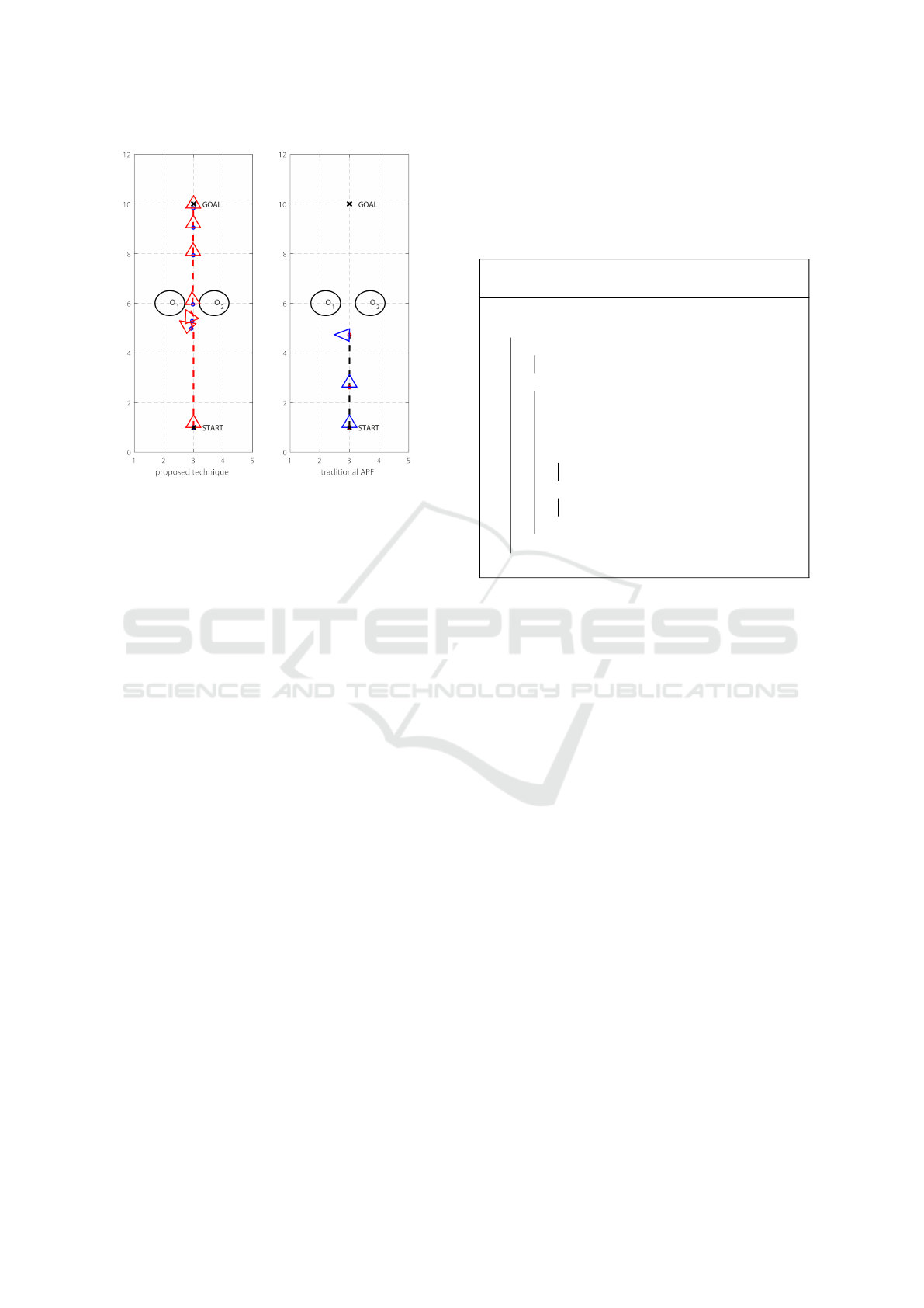
Figure 5: Proposed method (red robot on the left) versus
traditional APF (blue robot on the right).
3 is always tangent to the circle centered in the obsta-
cle of interest and passing by the robot pose. As a con-
sequence, if D = −∇U
b
(r(t),
˜
O) is the vector which
allows for bypassing the obstacle in a sense, the vec-
tor −D lets the robot be driven around the obstacle in
the reverse sense. Aiming at reaching the target using
the shortest path, the points
r
1
=

x
r
(t)
y
r
(t)

+ τD, r
2
=

x
r
(t)
y
r
(t)

− τD (9)
are computed, where τ is a small parameter, and de-
pending on the point r
j
, j = 1,2, nearest to G, in the
Euclidian sense, the bypassing verse is chosen.
In conclusion, the overall potentials selection
rules can be summarized by the algorithm 1.
Note that the proposed technique may suffer of
discontinuity in the negative gradient −∇U(r(t)) due
to the switching between potentials. If the plan-
ning requirements demand for a smooth path, com-
pliant with non-holonomic robot movements, the ob-
tained trajectory can be properly adapted by stop-
ping the robot at each switch and rotating it to the
direction imposed by the new negative gradient and
then starting the movement. Otherwise, −∇U(r(t
−
))
and −∇U(r(t)) may be linked by a properly chosen
smoothing function.
Remark 2. Note that in a standard configuration, the
use of a switching among two or more potentials may
not solve the local minima problem since it could be
possible that the potential fields create an oscillation
between the local minima yielding to a never ending
local minimum oscillation configuration. However,
since the obstacles are assumed to be static and the
proposed bypassing potential drives the robot around
the obstacle in clockwise or counterclockwise sense
depending only from the goal position and not from
the obstacles locations, the never ending oscillation
can not occur.
Algorithm 1: Artificial Potentials selection al-
gorithm, applied for each t ∈ R
+
input : Goal position G; robot pose r(t)
while G is not reached do
if @O
j
satisfying (7) then
U(r(t)) = U
a
(r(t),G);
else
˜
O =obstacle at minimum distance in
the tube T (r(t),G,R
m
);
compute r
1
and r
2
using Eq. (9);
if ||r
1
− G|| ≤ ||r
2
− G|| then
−∇U(r(t)) = D;
else
−∇U(r(t)) = −D;
end
end
end
Remark 3. According to the proposed method, a con-
vex/concave obstacle or a wall-like obstacle can be
avoided by considering the circumscribing circle in-
stead of the real obstacle shapes. In an alternative
way, this obstacle can be bypassed by using virtual
obstacles placed in the detected nearest obstacle part
and with the virtual radius equal to the actual dis-
tance from the robot to the detected obstacle portion.
Within this context, to avoid stall configurations, the
bypassing sense is a-priori chosen and used for all the
virtual obstacles related to the real one; the strategy
remains then the same.
5 CONTROL LAW
As explained in (Siciliano et al., 2008), the negative
gradient can be interpreted as a desired velocity for
the robot. Let now assume the robot can be modeled
by the standard non-holonomic model



˙x
r
(t) = v
r
(t)cos(θ
r
(t))
˙y
r
(t) = v
r
(t)sin(θ
r
(t))
˙
θ
r
(t) = ω
r
(t)
(10)
where v
r
(t) and ω
r
(t) are the robot linear and rota-
tional velocities respectively. Let v
∇
(t) = −∇U (r(t))
be the desired robot velocity, chosen using the pro-
posed path planning method, where M
v
= ||v
∇
(t)||,
θ
∇
= ∠v
∇
(t).
Path Planning and Obstacles Avoidance using Switching Potential Functions
347

Figure 6: Proposed method (red line) versus traditional APF
(blue line).
Theorem 1. The control law
v
r
(t) = M
v
cos(θ
∇
(t) − θ
r
(t)) (11)
ω
r
(t) = K
ω
(t)(θ
∇
(t) − θ
r
(t)) (12)
with
K
ω
(t) =











˙
θ
∇
(t) + K
c
(θ
∇
(t) − θ
r
(t))
θ
∇
(t) − θ
r
(t)
,
if |θ
∇
(t) − θ
r
(t)| > 0
0, otherwise;
(13)
where K
c
> 0 is a control tuning parameter, ensures
the robot to track the desired velocity v
∇
(t).
Proof. Consider the Lyapunov function
V (r(t)) =
1
2
(θ
∇
(t) − θ
r
(t))
2
(14)
with
˙
V (r(t)) = (θ
∇
(t) − θ
r
(t))(
˙
θ
∇
(t) −
˙
θ
r
(t)). (15)
Using Eqs. (10), (12) and (13) it follows that
˙
V (r(t)) = (θ
∇
(t) − θ
r
(t))(
˙
θ
∇
(t) − ω
r
(t)) =
= (θ
∇
(t) − θ
r
(t))(
˙
θ
∇
(t) − K
ω
(t)(θ
∇
(t) − θ
r
(t))) =
= −K
c
(θ
∇
(t) − θ
r
(t))
2
.
(16)
Since
˙
V (r(t)) < 0 ∀θ
r
(t) 6= θ
∇
(t), the proposed
control law ensures θ
r
(t) → θ
∇
(t) and, as a conse-
quence, ω
r
(t) → 0 and v
r
(t) → M
v
.
Remark 4. Note that, using the proposed control law,
the derivative of the Lyapunov function can be written
as
˙
V (r(t)) = −2K
c
V (r(t)) (17)
and then
V (r(t)) = e
−2K
c
t
V (r(0)) (18)
where V (r(0)) is the square of the angular error be-
tween the robot heading and the negative gradient an-
gle at the switching time. As a consequence, the tran-
sient time required by the control to ensure the error is
lower than a given error threshold, can be computed.
Remark 5. Since neither the attractive potential U
a
nor the bypassing potential U
b
depend on θ
r
(t), the
value
˙
θ
∇
(t) can be easily computed given the robot
current pose and the active potential field U(r(t)):
˙
θ
∇
(t) =
∂θ
∇
(t)
∂x
r
˙x
r
(t) +
∂θ
∇
(t)
∂y
r
˙y
r
(t),
where ˙x
r
(t), ˙y
r
(t) are given by Eqs. (8) and (11).
6 RESULTS
To evaluate the performance of the proposed path
planning and control technique, three numerical con-
figurations have been tested, using the following pa-
rameters
R
v
= 1.5m, R
i
= 0.5m ∀i, R
m
= 2m,
τ = 0.05, K
c
= 10, c = 1,
δ = 10
−4
,
and the traditional attractive potential
U
a
(r(t),G) =




G −

x
r
(t)
y
r
(t)





2
.
In the first two testing configurations, the de-
scribed new method has been contrasted with the tra-
ditional APF technique shown in (Siciliano et al.,
2008).
First of all, the proposed method has been tested
by placing the robot in [3,1]
T
with an initial head-
ing of θ
r
(0) =
π
2
and requiring to reach the goal
[x
G
,y
G
] = [3,10]
T
avoiding collisions with two obsta-
cles placed in [2.2,6]
T
and [3.7,6]
T
. The robot motion
in this context, using traditional APF or the proposed
path planning rules, is shown in Fig. 5.The traditional
method incurs in a local minima problem while the
proposed technique avoids this trouble thanks to the
use of a single artificial potential at time, switching it
between the attractive one and the bypassing one. The
robot is then driven between the two obstacles with no
stall configurations or collisions.
The second tested configuration consists in four
obstacles placed in [2.5,2.5]
T
, [5,1.5]
T
, [7,0.5]
T
,
[8,3]
T
. The robot starts its path from in [1,2]
T
with
an initial heading of θ
r
(0) = 0 and aims at reaching
[x
G
,y
G
] = [11,3]
T
. A comparison between traditional
APF and the proposed technique is depicted in Fig. 6.
Both the methods properly drive the robot to the goal.
ICINCO 2017 - 14th International Conference on Informatics in Control, Automation and Robotics
348

Figure 7: Proposed method when the environment contains
a large number of obstacles.
As expected, the use of a switching strategy yields to
a less smooth trajectory w.r.t. the one obtained by the
traditional APF method. Note that the proposed plan-
ning rules aim at driving the robot to the goal what-
ever is the obstacles configuration with no regards on
other trajectory optimality criteria. It follows that the
obtained robot path could be slower/faster or more
complicated w.r.t. the one obtained with other tech-
niques but, on the other hand, the proposed method
will always provide a solution to the target reaching
with obstacles avoiding problem.
In the third testing configuration, the robot has
been placed in [1,3]
T
with an initial heading of
θ
r
(0) = 0, the goal is in [x
G
,y
G
] = [10,3]
T
and a 16
obstacles, placed as shown in Fig. 7, have been used
to obstruct the robot movements. This testing con-
figuration proposes various local minima situations in
the traditional APF case. For example, if the obstacle
O
16
is equipped with a traditional artificial repulsive
potential, it could prevent the robot from reaching the
goal due to the imposed repulsion when the robot is
close to its target. On the contrary, using the proposed
planning method, the robot is driven to the goal with
no local minima situations and avoiding all the obsta-
cles in the environment, as shown in Fig. 7. In partic-
ular, obstacle O
16
does not affect robot path since it is
placed after the goal, in the robot point of view, and
as a consequence it is out of the tube T (r(t),G,R
m
).
7 CONCLUSIONS
In this work, a novel approach to the artificial poten-
tials method has been proposed to face the path plan-
ning and obstacles avoidance problem for a mobile
robot. The new method has been developed aiming
at overcoming the well known local minima problem
of the traditional APF technique. A novel helicoidal
potential has been proposed to allow for bypassing
an obstacle using only the effect of a single potential
field, with no need for the summation of a repulsive
one and an attractive one, in order to avoid local min-
ima. In this context, the proposed method is based
on the use of a single potential at a time, switching
from attractive to bypassing case depending on a set
of defined switching rules.
Moreover, since only local information is used,
the proposed technique ensures high robustness, in
terms of achieved performance and computational
complexity, w.r.t. the number of obstacles.
The described method has been compared, in a nu-
merical way, with traditional APF technique, and has
shown a more robust behavior w.r.t. it, providing a
feasible path to the robot goal also in the case of a
framework with multiple obstacles to be avoided.
As a future research direction, the proposed tech-
nique will be extended to the case of mobile obstacles.
REFERENCES
Alajlan, M., Kouba, A., Chari, I., Bennaceur, H., and Am-
mar, A. (2013). Global path planning for mobile
robots in large-scale grid environments using genetic
algorithms. In 2013 International Conference on In-
dividual and Collective Behaviors in Robotics (ICBR),
pages 1–8.
Araujo (2006). Prune-able fuzzy art neural architecture for
robot map learning and navigation in dynamic envi-
ronments. IEEE Transactions on Neural Networks,
17(5):1235–1249.
Benzerrouk, A., Adouane, L., and Martinet, P. (2012). Dy-
namic obstacle avoidance strategies using limit cycle
for the navigation of multi-robot system. In IEEE/RSJ
International Conference on Intelligent Robots and
Systems, 4th Workshop on Planning, Perception and
Navigation for Intelligent Vehicles.
Bi, Z., Yimin, Y., and Wei, Y. (2008). Hierarchical path
planning approach for mobile robot navigation under
the dynamic environment. In 2008 6th IEEE Inter-
national Conference on Industrial Informatics, pages
372–376.
Bopardikar, S. D., Englot, B., and Speranzon, A. (2015).
Multiobjective path planning: Localization con-
straints and collision probability. IEEE Transactions
on Robotics, 31(3):562–577.
Chamberland, S., Beaudry, ., Clavien, L., Kabanza, F.,
Michaud, F., and Lauriay, M. (2010). Motion plan-
ning for an omnidirectional robot with steering con-
straints. In 2010 IEEE/RSJ International Conference
on Intelligent Robots and Systems, pages 4305–4310.
Choset, H., Lynch, K. M., Hutchinson, S., Kantor, G. A.,
Burgard, W., Kavraki, L. E., and Thrun, S. (2005).
Principles of Robot Motion: Theory, Algorithms, and
Implementations. MIT Press, Cambridge, MA.
Path Planning and Obstacles Avoidance using Switching Potential Functions
349

Chu, K., Lee, M., and Sunwoo, M. (2012). Local path plan-
ning for off-road autonomous driving with avoidance
of static obstacles. IEEE Transactions on Intelligent
Transportation Systems, 13(4):1599–1616.
Franz
`
e, G. and Lucia, W. (2015). The obstacle avoidance
motion planning problem for autonomous vehicles: A
low-demanding receding horizon control scheme. Sys-
tems & Control Letters, 77:1 – 10.
Franz
`
e, G. and Lucia, W. (2016). A receding horizon con-
trol strategy for autonomous vehicles in dynamic en-
vironments. IEEE Transactions on Control Systems
Technology, 24(2):695–702.
Khatib, O. (1990). Real-Time Obstacle Avoidance for
Manipulators and Mobile Robots, pages 396–404.
Springer New York.
Kim, D.-H. and Kim, J.-H. (2003). A real-time limit-cycle
navigation method for fast mobile robots and its ap-
plication to robot soccer. Robotics and Autonomous
Systems, 42(1):17 – 30.
Lau, B., Sprunk, C., and Burgard, W. (2013). Efficient
grid-based spatial representations for robot naviga-
tion in dynamic environments. Robotics and Au-
tonomous Systems, 61(10):1116 – 1130. Selected Pa-
pers from the 5th European Conference on Mobile
Robots (ECMR 2011).
Mac, T. T., Copot, C., Tran, D. T., and De Keyser, R. (2016).
Heuristic approaches in robot path planning. Robot.
Auton. Syst., 86(C):13–28.
Park, M. G. and Lee, M. C. (2003). A new technique
to escape local minimum in artificial potential field
based path planning. KSME International Journal,
17(12):1876–1885.
Rosell, J. and Iniguez, P. (2005). Path planning using
harmonic functions and probabilistic cell decomposi-
tion. In Proceedings of the 2005 IEEE International
Conference on Robotics and Automation, pages 1803–
1808.
ˇ
Seda, M. (2007). Roadmap methods vs. cell decomposi-
tion in robot motion planning. In Proceedings of the
6th WSEAS International Conference on Signal Pro-
cessing, Robotics and Automation, pages 127–132.
World Scientific and Engineering Academy and So-
ciety (WSEAS).
Siciliano, B., Sciavicco, L., Villani, L., and Oriolo, G.
(2008). Robotics: Modelling, Planning and Control.
Springer Publishing Company, Incorporated, 1st edi-
tion.
Struik, D. (1961). Lectures on Classical Differential
Geometry. Addison-Wesley series in mathematics.
Addison-Wesley Publishing Company.
Yang, S. X. and Meng, M. (2000). An efficient neural
network approach to dynamic robot motion planning.
Neural Networks, 13(2):143 – 148.
Zhang, H., Butzke, J., and Likhachev, M. (2012). Combin-
ing global and local planning with guarantees on com-
pleteness. In Robotics and Automation (ICRA), 2012
IEEE International Conference on, pages 4500–4506.
IEEE.
ICINCO 2017 - 14th International Conference on Informatics in Control, Automation and Robotics
350