Framework for Fair Comparisons of Underwater Vehicle Controllers

Showcasing the Robustness Properties of a Model-free Sliding Mode Controller

Tuned with a Random-forest-based Bayesian Optimization Approach

Musa Morena Marcusso Manh

aes

, Sebastian A. Scherer

, Luiz Ricardo Douat

Martin Voss

and Thomas Rauschenbach

Corporate Sector for Research and Advance Engineering, Robert Bosch GmbH,

Robert-Bosch-Campus 1, 71272, Renningen, Baden-W

urttemberg, Germany

Advanced System Technology (AST), Fraunhofer-Institute of Optronics, Systems Technologies and Image Exploitation,

Am Vogelherd 50, 98693, Ilmenau, Th

uringen, Germany

Keywords:

Underwater Robotics, Robust Control, Parameter Optimization, Sliding Mode Control, SMAC, Underwater

Robotics Simulation, Gazebo.

Abstract:

Tasks with underwater vehicles present several challenges that include complex and hazardous environments,

and unmodeled and/or unknown uncertainties. The setup of positioning controllers is therefore a difﬁcult and

laborious task and very often leads to suboptimal performance results on the ﬁeld. This paper shows a frame-

work for methodical evaluation and setup of dynamic positioning controllers for underwater vehicles with

simulation-based optimization method using performance metrics. The proposed method can be conﬁgured

to be mission speciﬁc and delivers a controller conﬁguration that also allows a fair numerical comparison

between control algorithms on similar scenarios.

1 INTRODUCTION

From underwater inspection of off-shore wind turbine

structures in depths of a few dozen meters to oil and

gas interventions in thousands of meters, remotely op-

erated vehicles (ROVs) constitute an ubiquitous en-

abler of industrial subsea activities.

The specialized literature provides several ad-

vanced model-based control strategies for underwater

vehicles (Fossen, 2011; Zhu and Gu, 2011; Molero

et al., 2011; Khadhraoui et al., 2014; Soylu et al.,

2016). Nevertheless, many algorithms still rely

on PID-like controllers due to their simple imple-

mentation (Hosseini and Seyedtabaii, 2016; Garcia-

Valdovinos et al., 2009). PID controllers can be eas-

ily tuned even when the vehicle model is unknown,

but at the expense of not intrinsically assuring robust-

ness properties against system parameter variations

and external disturbances. A promising model-free

robust alternative, based on variable structure sliding

mode control, was presented in (Garc

ıa-Valdovinos

et al., 2014).

In (Garc

ıa-Valdovinos et al., 2014), as well as in

numerous other sources in the same ﬁeld, the pro-

posed controller has its parameters selected follow-

ing a trial and error procedure, which not only can-

not guarantee a good performance in the presence of

uncertain perturbations but also makes the numeri-

cal comparison with other dynamic positioning con-

trollers, even under equal scenarios, rather difﬁcult

(Antonelli, 2014). Furthermore, considering the dif-

ﬁcult environment in which underwater vehicles have

to be deployed regarding costs and sensor systems, a

preliminary simulation-based evaluation can be used

to decrease the number of iterations on experiments

related to controller conﬁguration by providing a pa-

rameter set that has shown good performance metrics

in simulated scenarios.

To the best knowledge of the authors, there are to-

day no published results on optimal parameter search

applied to dynamic positioning controllers with par-

ticular focus on performance analysis, but exam-

ples can be found in other ﬁelds such as for safe

optimization of controller parameters for quadrotors

(Berkenkamp et al., 2016) and gait optimization for

bipedal locomotion (Calandra et al., 2014). Both

(Berkenkamp et al., 2016) and (Calandra et al., 2014)

rely on Gaussian processes to learn the system’s per-

formance metrics from a set of experimental data and

use this ﬁtted model in the search for optimal param-

102

Manhães, M., Scherer, S., Douat, L., Voss, M. and Rauschenbach, T.

Framework for Fair Comparisons of Underwater Vehicle Controllers - Showcasing the Robustness Properties of a Model-free Sliding Mode Controller Tuned with a Random-forest-based

Bayesian Optimization Approach.

DOI: 10.5220/0006427001020113

In Proceedings of the 7th International Conference on Simulation and Modeling Methodologies, Technologies and Applications (SIMULTECH 2017), pages 102-113

ISBN: 978-989-758-265-3

eters for the system’s controller and walking gait. As

discussed in (Calandra et al., 2014), the strategy has

been shown to converge to a near-optimal solution us-

ing a much smaller number of system runs in compar-

ison with algorithms that rely, for example, on gradi-

ent descent methods.

The objective of this paper is to create a method-

ical simulation-based procedure to search for the op-

timal parameter set for a generic controller through

minimization of a performance cost function to en-

able a fair comparison of dynamic positioning con-

trollers in equal scenarios and mission plan. The

minimizer used for the parameter search, SMAC

(”Sequential Model-based Algorithm Conﬁguration”)

(Hutter et al., 2011; Lindauer et al., 2017), ﬁts a ran-

dom forest model on data extracted from the perfor-

mance cost function computed after each simulation

run to search for best controller parameter set.

The performance cost function is based on perfor-

mance metrics that are derived from simulated pose

and velocity error in a scenario where the vehicle is

subjected to different types of disturbances while fol-

lowing a pre-deﬁned trajectory. The objective is to

ﬁnd parameters that will allow the vehicle to com-

plete a mission with focus on the performance for tra-

jectory tracking and disturbance rejection. The con-

trollers to be parametrized and later compared against

each other for the use-case presented in this paper are

a conventional MIMO PID controller and a model-

free sliding mode controller (Garc

ıa-Valdovinos et al.,

2014). Both were implemented using ROS and in-

tegrated into the UUV Simulator (Manh

aes et al.,

2016a) to control a fully actuated work-class ROV.

The paper is further structured as follows. In Sec-

tion 2 an overview of the controller optimization is de-

picted. The controllers used in this use-case are pre-

sented in Section 3. The simulated scenario is shown

in detail in Section 4. The results for the optimal con-

troller parametrization are presented in 5 and a vali-

dation experiment for a different scenario is presented

in 6. Section 7 includes conclusion and discussion of

the results. The source code and the simulation envi-

ronment used to generate the results presented in the

following sections can be found at (Manh

aes et al.,

2016a).

2 PERFORMANCE-BASED

CONTROLLER

PARAMETRIZATION

Performance analysis to evaluate controllers is al-

ready a subject of interest in ﬁelds with hard security

Initial parameter set Θ

Trajectory (η

)) for i ∈ [0, N]

Disturbance models D

for k ∈ [1, N

]

Performance metrics M

for m ∈ [1, N

]

Run simulation with Θ

Compute performance metrics M

from

error sets and control eﬀort

Compute performance cost function

Update optimizer

Update best parameter

set candidate Θ

∗

Compute parameter set Θ

n+1

Optimal parameter set

∗

selected

n = n + 1

End

Figure 1: Flow chart to the parameter optimization proce-

dure.

constraints, such as ﬂight control (Heise et al., 2013;

Stepanyan et al., 2009). The procedure is indepen-

dent of the system model and controller algorithm,

and tries to guarantee that the system will present a

safe performance during its tasks. The establishment

of a clear method for controller design and evaluation

can also beneﬁt the creation of safety and control de-

sign standards (Stepanyan et al., 2009).

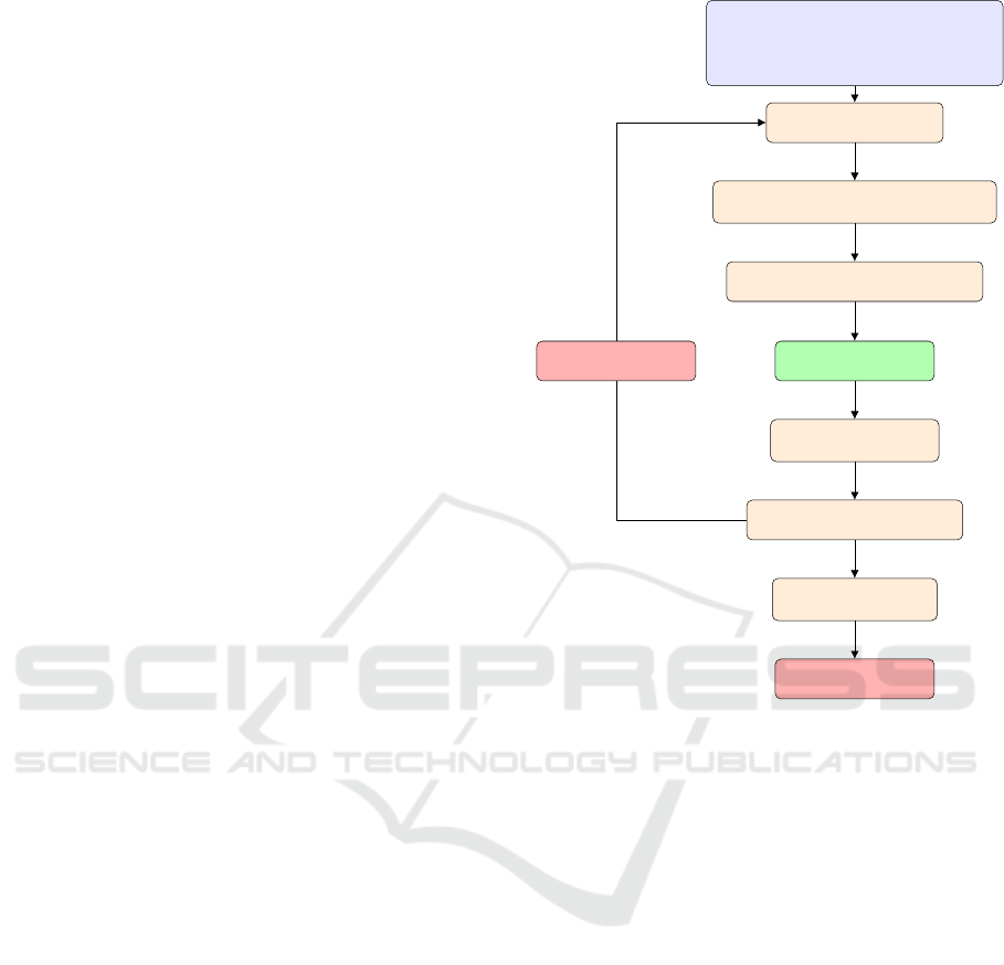
As shown in Figure 1, the procedure is very

straightforward. The parameter optimization is exe-

cuted for a speciﬁc scenario using pre-deﬁned distur-

bances models D

. The disturbance models are cho-

sen in order to represent a worst case scenario for the

mission objective in order to allow the optimal param-

eter set to provide a good trajectory tracking perfor-

mance for a large range of unmodeled disturbances.

There is, however, the possibility of controller pa-

rameters converging to a local minima without ex-

ploring the parameter set or the resulting set will be

a result of overﬁtting the controller parameters to

the given simulated scenario. It was therefore de-

cided upon the use of the algorithm conﬁguration tool

SMAC (Hutter et al., 2011). This global black-box al-

Framework for Fair Comparisons of Underwater Vehicle Controllers - Showcasing the Robustness Properties of a Model-free Sliding Mode

Controller Tuned with a Random-forest-based Bayesian Optimization Approach

103

gorithm conﬁguration method calculates the next pa-

rameter sets by ﬁtting a random forest model to the

deﬁned cost function output. Due to the use of ran-

dom forest models, the optimizer is less likely to get

stuck in local minima and is capable of exploring un-

seen regions of the parameter space (Hutter et al.,

2011).

2.1 Performance Cost Function

The performance of a controller applied to a scenario

is a very broad subject to tackle and highly dependent

on the application and/or mission. For this use-case,

the performance metrics used are focused on the po-

sition and orientation errors. Considering a trajectory

(η

)) for i ∈ [0,N] and t

being the ﬁnal time

stamp, set as reference for pose (η

) and velocity (

)

to the controller, pose and velocity error vectors can

be computed after each simulated scenario with a con-

troller parameter set Θ

The cost function takes then into account a

weighted sum of root mean square errors for position

and orientation as shown in Equation 1:

∑

m=1

∑

i=0



) − η

))



+ w

∑

i=0

(φ

) − φ(t

))

+ w

∑

i=0

(θ

) − θ(t

))

+ w

∑

i=0

(ψ

) − ψ(t

))

(1)

being w

set as the inverse of the maximum accepted

value for the metrics in case, η

the reference posi-

tion vector (x

)

, and φ

, θ

and ψ

the orien-

tation reference in roll, pitch and yaw, respectively.

2.2 Disturbance Models

Two types of disturbance models are considered in

this paper. The ﬁrst basic model is the application

of wrench vector deﬁned on the WORLD frame to

the vehicle’s center of mass for a limited time range

]. The disturbance can be formally described in

Equation 2.

F =

(

,τ

)

, for t

≤ t ≤ t

0 ∈ R

, otherwise

(2)

In a similar way, a constant current velocity V

also deﬁned in the WORLD frame subject to the hor-

izontal angle θ

can also be scheduled to be added

to the simulation for a given time range in a similar

manner following the model in Eq. 3.

(

cosθ

sinθ

,0)

, for t

≤ t ≤ t

0 ∈ R

, otherwise

(3)

3 CONTROLLERS

In this study case, two model-free controllers were

subject to parameter optimization: a conventional

MIMO PID controller and a model-free sliding mode

controller. Both controllers were optimized in the

same scenario with the same disturbances to allow a

fair comparison later on.

3.1 MIMO PID Controller

Consider ξ and

ξ to be, respectively, the pose and ve-

locity error vectors in R

with respect to the BODY-

frame, the PID controller’s control force output is de-

scribed by the following equation:

PID

= K

ξ + K

ξ(τ)dτ (4)

where K

∈ R

6×6

are chosen to be positive

semi-deﬁnite diagonal matrices.

3.2 Model-free Sliding Mode Controller

The model-free sliding mode controller presented be-

low is based on the work of (Garc

ıa-Valdovinos et al.,

2014) but differs in two aspects from the original al-

gorithm, namely that the errors are represented in the

BODY-frame coordinates and, according to our con-

vention, errors are represented with the opposite sign.

Assume BODY-frame velocities and WORLD-

frame poses to be represented, respectively, as

ν = [ν

,ν

]

= [u,v, w, p,q,r]

and η = [η

,η

]

[x,y,z,φ,θ,ψ]

, where ν

∈ R

and ν

∈ R

are the

linear and angular velocity vectors with respect to the

BODY-frame, and η

∈ R

and η

∈ R

are position

and orientation vectors represented in the WORLD-

frame.

The equation of motion expressed in BODY-frame

(Fossen, 2011) is given as:

ν + C(ν)ν + D(ν)ν + g(η) = τ

(5)

with M ∈ R

6×6

, C ∈ R

6×6

, D ∈ R

6×6

, g ∈ R

, and

τ ∈ R

representing respectively the inertia and added

SIMULTECH 2017 - 7th International Conference on Simulation and Modeling Methodologies, Technologies and Applications

104

mass matrix, the Coriolis and centripetal terms ac-

counting with added mass terms, the damping matrix,

the gravitational forces and the control inputs. The

transformation

η = J(η)ν is used to convert linear and

angular velocity from BODY to WORLD frame, J(η)

being deﬁned as in (Garcia-Valdovinos et al., 2009).

The left-hand side of Equation 5 can be linearly

parametrized, in terms of a nominal reference (ν

by the product of a regressor Y

(ν,η,ν

) ∈ R

6×p

(Lantos and M

arton, 2011), composed of known non-

linear terms, and a constant parameter vector Θ ∈ R

+ C(ν)ν

+ D(ν)ν

+ g(η) = Y

(ν,η,ν

)Θ

(6)

Subtracting (6) from (5) leads to the representa-

tion of Equation 5 in error coordinates (Parra-Vega

and Arimoto, 1995; Garc

ıa-Valdovinos et al., 2014):

+ C(ν)s

+ D(ν)s

= τ − Y

(ν,η,ν

)Θ (7)

with the extended error s

= ν − ν

Deﬁning a change of coordinates to the nominal

reference (Parra-Vega et al., 2003; Garc

ıa-Valdovinos

et al., 2014) leads to:

= ν

+ αξ + s

− K

sign(s

)dσ (8)

where

= s(t

−κt

(9)

= s − s

(10)

with α and K

being diagonal positive deﬁnite 6 × 6

matrices, κ a positive scalar, sign(x) the input-wise

discontinuous signum function for the vector x, and

the sliding surface s deﬁned as s = −

ξ − αξ. s

is re-

sponsible for a smooth initialization of the controller

output and ν

is the velocity reference with respect to

the BODY frame. The extended error s

can be writ-

ten as:

= s

+ K

sign(s

)dσ (11)

The control law τ

= −K

, with K

as a diag-

onal positive 6 ×6 matrix, in closed-loop with system

presented in Equation 7 yields to:

= − K

− C(ν)s

− D(ν)s

− Y

(ν,ν

,η)Θ.

(12)

To ensure the convergence of the system, let us

consider a Lyapunov candidate function deﬁned as

follows, as given by (Garcia-Valdovinos et al., 2009):

V =

(13)

Its corresponding time derivative is:

V =s

[−K

− C(ν)s

− D(ν)s

− Y

Θ]+

(14)

Now, using the fact that x

[

M−2C(ν)]x = 0, ∀x ∈

, x 6= 0, we have:

V = −s

+ D(ν)]s

− s

Θ (15)

Since D(ν) is a positive deﬁnite matrix and Y

is upper bounded (Parra-Vega et al., 2003) by ρ(t):

V = −s

+ D(ν)]s

− s

≤ −s

− s

≤ −s

ρ(t)

(16)

Equation 16 allows to conclude that for sufﬁ-

ciently large K

values and small initial error con-

ditions, the time derivative of the Lyapunov function

is negative semideﬁnite, implying converge of s

to a

set-bounded set ε, i.e. s

→ ε as t → ∞. Rewriting

Equation 12 as:

= − M

−1

+ C(ν)s

+ D(ν)s

+ Y

(ν,ν

,η)Θ]

(17)

and using the fact that all right-hand side terms of this

equation are upper bounded (Parra-Vega et al., 2003),

it follows that:

≤ ε

(18)

Now, deriving Equation 11 and rearranging the

terms:

= −K

sign(s

) +

(19)

Multiplying Equation 19 by s

= −s

sign(s

) + s

≤ −λ

min

)



≤



(−λ

min

) + ε

)

≤ −µ



(20)

min

) > ε

→ µ > 0, assuring sliding mode at

≤ (|s

)/µ|) and, since s

) = 0 for any initial

condition, sliding mode in s

(t) = 0 is enforced for

all time.

From Equation 9, s

→ 0 exponentially, and from

Equation 10:

= −

ξ − αξ − s

⇒

ξ = −αξ (21)

Framework for Fair Comparisons of Underwater Vehicle Controllers - Showcasing the Robustness Properties of a Model-free Sliding Mode

Controller Tuned with a Random-forest-based Bayesian Optimization Approach

105

implying exponential convergence of the tracking er-

rors. The full control law after s

converges to zero

after initialization is shown in Equation 22.

= K

αξ + K

ξ + K

sign(

ξ + αξ)dσ

(22)

4 SIMULATION SCENARIO

DESCRIPTION

The simulation was built and conﬁgured using

the UUV Simulator (Manh

aes et al., 2016b), an

open-source underwater simulation package for the

robotics simulator Gazebo (Koenig and Howard,

2004) using ROS (”Robot Operating System”) as a

system application and communication framework.

The simulator is built in a modular fashion, which al-

lows an easy setup of the scenarios for different con-

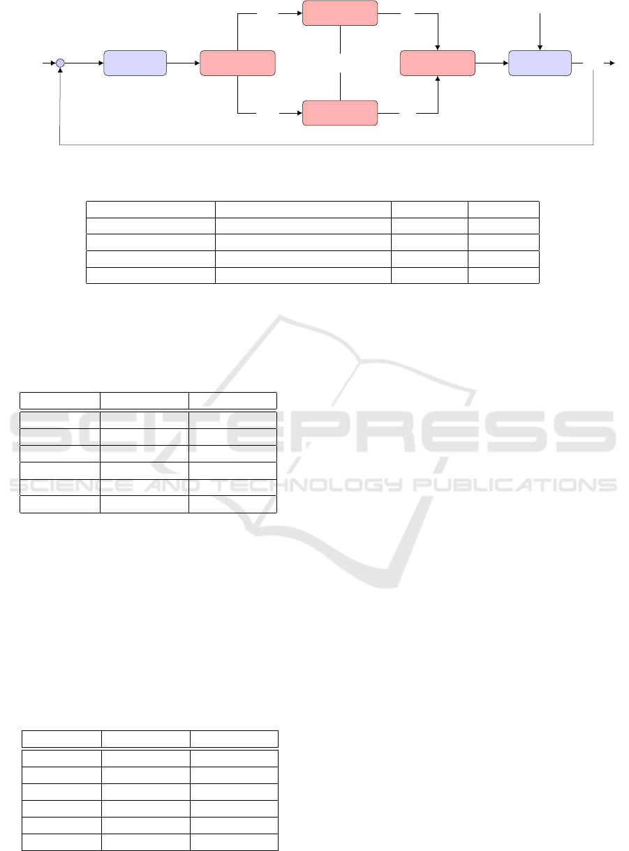
troller algorithms. The information ﬂow between the

modules is shown in Figure 3. A view of the 3D vi-

sualization tool during the simulation of the scenario

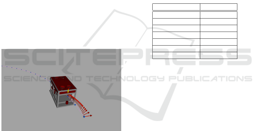
with the test trajectory is shown in Figure 2.

Figure 2: Snapshot from the RViz environment (ROS 3D vi-

sualization tool) for the ﬁrst few seconds after the trajectory

following started. The red arrows show the heading for past

samples and the pink line represents the path to be followed.

4.1 Vehicle Model

The vehicle considered in this paper is a fully actu-

ated work-class ROV with parameters retrieved from

(Berg, 2012) based on the Sperre SF 30k ROV with

a slightly different thruster conﬁguration and thruster

models. The vehicle’s dynamic model, visual and col-

lision geometries can be found as part of the UUV

Simulator package (Manh

aes et al., 2016b).

The thruster units (see Figure 3) include a steady-

state curve described by τ

= 0.00031|Ω|Ω, where

Ω is the rotor’s angular velocity, and a ﬁrst-order

dynamic model to represent the propeller dynamics

(Manh

aes et al., 2016a). Ω

is the rotor command

velocity is obtained through the inverse of the steady-

state angular velocity to thrust function applied to the

desired thrust force τ

4.2 Trajectory and Disturbances

The pose and velocity reference were computed from

a helical trajectory. The WORLD frame follows in

this case the ENU (East-North-Up) convention since

it is the standard for the Gazebo simulator, and is

therefore the reference frame for the trajectory gener-

ated. The trajectory parameters are listed in Table 1.

Table 1: Reference trajectory parameterized with the con-

troller benchmark.

Parameter Value

Type of trajectory Helical

Radius 20 m

∆z 10 m

# of turns 2

Duration 200 s

Center point (0,0,−20) m

Start time 5 s

The disturbances are scheduled and generated by a

disturbance manager node using the models described

in Section 2.2 with respect to Gazebo’s WORLD

frame in the ENU convention. The disturbance model

description and their respective activation and deacti-

vation times can be seen in Table 2.

4.3 Controller Parameter Optimization

A fair comparison of the performance properties

of a PID and a model-free sliding mode con-

trol is proposed, where both controller parameters

are optimized using SMAC (Hutter et al., 2011),

a random-forest-based Bayesian optimization algo-

rithm. Bayesian optimization approaches are an ad-

equate choice when the cost function evaluations are

expensive to obtain (Brochu et al., 2010).

For both the controllers the SMAC task had to be

conﬁgured with the controller parameters, its ranges

and initial values, the cost function and the maximum

number of simulation runs. In both cases, the maxi-

mum number of simulation runs was set to 130. The

initial values for both controllers have been chosen to

deliver a stable closed-loop system.

For the MIMO PID controller presented in Section

3.1, the parameter matrices are deﬁned in Equation

SIMULTECH 2017 - 7th International Conference on Simulation and Modeling Methodologies, Technologies and Applications

106

Controller

Thruster

manager

Thruster unit 0

Thruster unit N

Thruster

allocator

Vehicle

system

ξ,

Ω

Disturbances

η,

−

Figure 3: Information ﬂow using the simulation environment.

Table 2: Parameters for the disturbance models used in the optimization process.

Disturbance model Value Start time End time

Wrench (3000 N,0,−3000 N,0,0,0) 25 s 75 s

Current (1.2,0,0) m/s 75 s 125 s

Wrench (0,0,0,0,0,3000 Nm) 125 s 150 s

Wrench (0,0,0,0,0,−3000 Nm) 150 s 175 s

23. The parameter search ranges and initial values are

listed in Table 3.

Table 3: Conﬁguration parameters for the MIMO PID pa-

rameter optimization.

Parameter Range Initial value

lin

[100, 20000] 5000

ang

[100, 20000] 5000

lin

[0, 5000] 0

ang

[0, 5000] 0

lin

[0, 20000] 0

ang

[0, 20000] 0

= diag(K

lin

3×3

ang

3×3

)

= diag(K

lin

3×3

ang

3×3

)

= diag(K

lin

3×3

ang

3×3

)

(23)

The model-free sliding mode controller described

in Section 3.2 has its matrices deﬁned as shown in

Equation 24. The setup used for SMAC is listed in

Table 4.

Table 4: Conﬁguration parameters for the model-free slid-

ing mode parameter optimization.

Parameter Range Initial value

lin

[100, 10000] 2000

ang

[100, 10000] 200

lin

[0, 10] 0.005

ang

[0, 10] 0.3

lin

[0.01, 5] 1.5

ang

[0.01, 5] 1.5

κ = 5

= diag(K

lin

3×3

ang

3×3

)

= diag(K

lin

3×3

ang

3×3

)

α = diag(α

lin

3×3

,α

ang

3×3

)

(24)

5 PARAMETRIZATION RESULTS

For the parametrization process, a task scheduler was

used to start all needed processes at each optimizer

iteration with the new set of parameters and process

the simulated data for the computation of the perfor-

mance metrics needed in the cost function described

in Section 2.1. The vehicle starts at the position

(x,y,z) = (20,0,−20) m in the ENU frame of the

Gazebo simulator world and with initial orientation

set as (φ,θ,ψ) = (0,0, 0) rad, with a initial heading

error of π/2 rad with respect to the initial trajectory

reference heading.

SMAC does not have a stopping criteria, it will

therefore search for the best parameter set until the

maximum number of simulation runs is reached, stor-

ing partial results during the process.

The weights of the cost function depicted in Sec-

tion 2.1 was set as w

= 1/RMSE

MAX

, RMSE

MAX

be-

ing an stipulated maximum acceptable value for the

corresponding metric. The weight values used in

the cost function according to the nomenclature used

in Section 2.1 are w

= 1/5 m

-1

, w

= 10/π rad

-1

= 10/π rad

-1

and w

= 6/π rad

-1

Framework for Fair Comparisons of Underwater Vehicle Controllers - Showcasing the Robustness Properties of a Model-free Sliding Mode

Controller Tuned with a Random-forest-based Bayesian Optimization Approach

107

5.1 MIMO PID Controller

Parametrization

The optimal controller parameters were found with a

corresponding cost function derived from SMAC’s ﬁt-

ted model of C

∗

PID

= 0.66059 after 28 evaluations, 1.8

hours after the optimizer was started (see Figure 4).

The controller parameters found are listed in Table 5.

Table 5: Optimal parameters for the MIMO PID controller

after optimization with SMAC.

Parameter Optimal values

lin

11993.888

ang

19460.069

lin

321.417

ang

2096.951

lin

9077.459

ang

18880.925

0 5 10 15 20 25

Number of evaluations

1.0

1.5

2.0

2.5

Cost function

Figure 4: Evolution of performance cost function for the

MIMO PID controller.

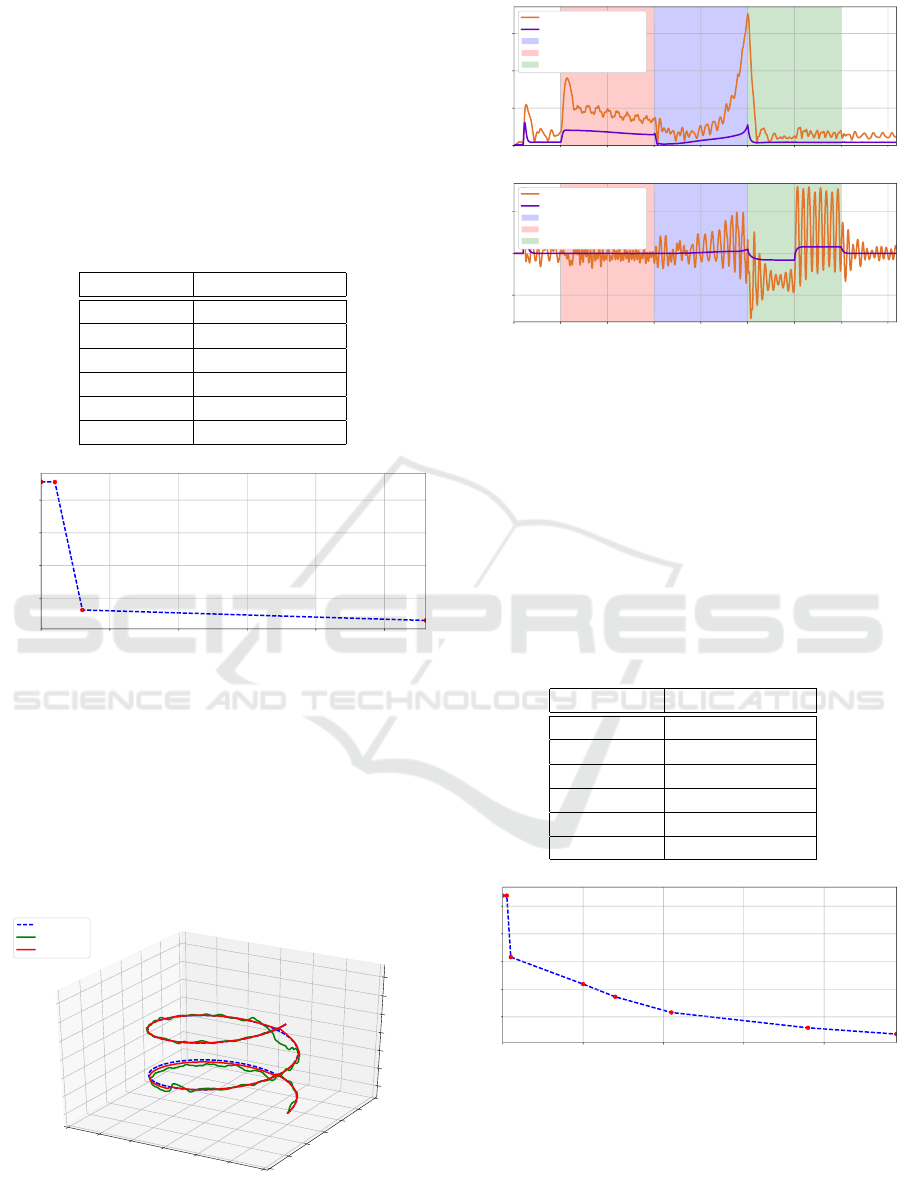
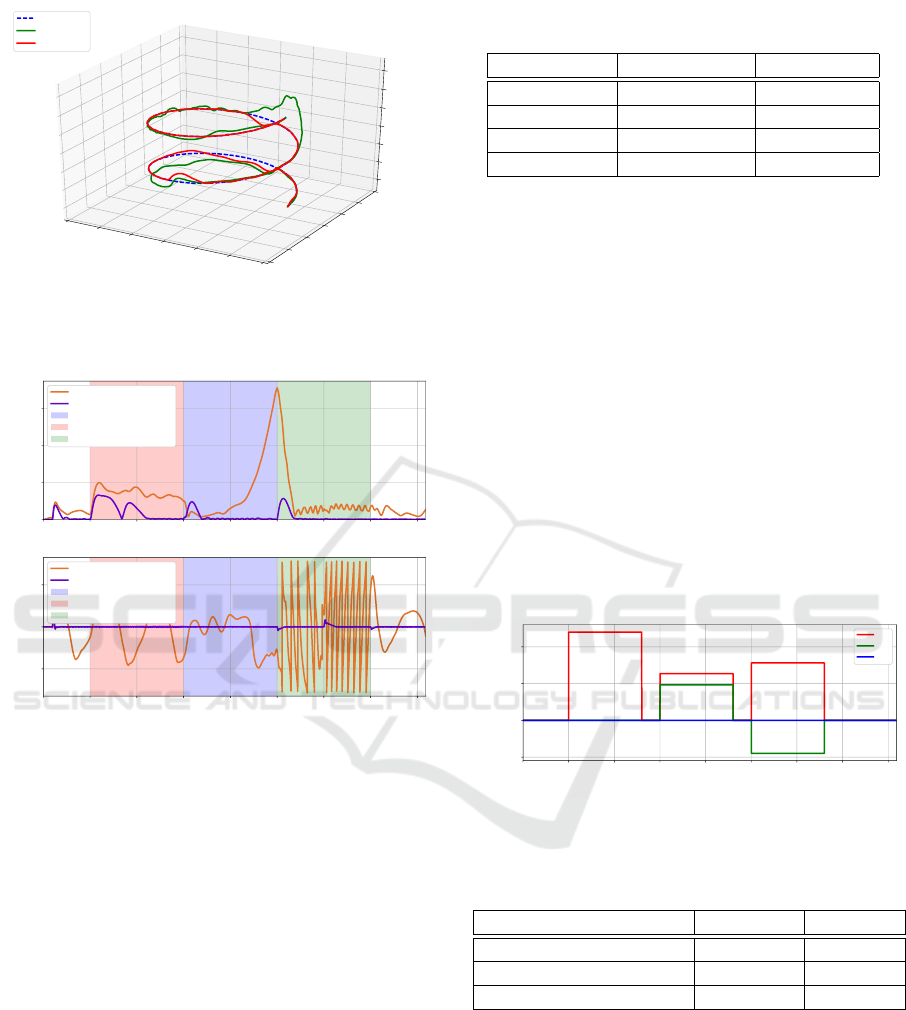
In Figure 5, the paths generated with the initial

and optimal parameter sets are compared against the

reference path. It illustrates the improvement of the

vehicle during its trajectory tracking task even in the

presence of disturbances. The position and heading

error curves for initial and optimal parameter sets are

shown in Figure 6.

X [m]

−30

−20

−10

Y [m]

−30

−20

−10

Z [m]

−20

−18

−16

−14

−12

−10

−8

Desired path

Initial set

Optimal set

Figure 5: Comparison between desired and actual trajecto-

ries for the initial and optimal parameter sets for the MIMO

PID controller under the inﬂuence of disturbances.

0 25 50 75 100 125 150 175 200

Time [s]

Position error [m]

Initial set

Optimal set

Current disturbance activated

Force disturbance activated

Torque disturbance activated

0 25 50 75 100 125 150 175 200

Time [s]

−1

Heading error [rad]

Initial set

Optimal set

Current disturbance activated

Force disturbance activated

Torque disturbance activated

Figure 6: Error curves for the best parameter set for the

MIMO PID controller.

5.2 Model-free Sliding Mode Controller

Parametrization

The optimal controller parameters were found with a

corresponding cost function being C

∗

= 0.378156

after 98 evaluations, 6.52 hours after the optimizer

was started (see Figure 7). The controller parameters

found are listed in Table 6.

Table 6: Optimal parameters for the model-free sliding

mode controller after optimization with SMAC.

Parameter Optimal values

lin

3243.315

ang

5602.003

lin

0.134

ang

0.169

lin

0.733

ang

4.833

0 20 40 60 80

Number of evaluations

Cost function

Figure 7: Evolution of the performance cost function for the

model-free sliding mode controller.

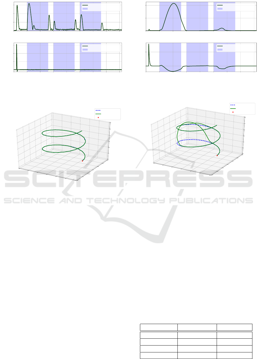
In Figure 8, the paths generated with the initial

and optimal parameter sets are compared with the ref-

erence path. The position and heading errors for both

the optimal and initial controller parameter sets can

be seen in Figure 9.

SIMULTECH 2017 - 7th International Conference on Simulation and Modeling Methodologies, Technologies and Applications

108

X [m]

−30

−20

−10

Y [m]

−30

−20

−10

Z [m]

−20

−18

−16

−14

−12

−10

−8

Desired path

Initial set

Optimal set

Figure 8: Comparison between desired and actual paths for

the initial and optimal parameter sets for the model-free

sliding mode controller under the inﬂuence of disturbances.

0 25 50 75 100 125 150 175 200

Time [s]

Position error [m]

Initial set

Optimal set

Current disturbance activated

Force disturbance activated

Torque disturbance activated

0 25 50 75 100 125 150 175 200

Time [s]

−2

Heading error [rad]

Initial set

Optimal set

Current disturbance activated

Force disturbance activated

Torque disturbance activated

Figure 9: Position error for the best and initial parameter set

for the model-free sliding mode controller under the inﬂu-

ence of disturbances.

5.3 Comparison of the Resulting

Optimized Controller Performances

Upon running both resulting parameter sets in the

simulated scenario, the performance metrics used for

the computation of the cost function (see Section 2.1)

for each use-case using the optimized controller pa-

rameters are presented in Table 7. The cost func-

tion computed from using the data Table 7 may differ

slightly from the SMAC’s output presented in Sec-

tions 5.1 and 5.2 since they were computed from its

calculated model.

Upon analysis of the generated paths and perfor-

mance metrics, both controllers achieve good results

both for position and heading tracking in the presence

of disturbances, with the PID controller test show-

ing a better position tracking performance and lower

maximum position error (see Figures 6 and 9). It is,

Table 7: Comparison of performance metrics after simula-

tion runs using the optimized controller parameters.

Metric Sliding Mode MIMO PID

RMSE

[m] 0.411 0.212

RMSE

[rad] 0.009 0.014

RMSE

[rad] 0.306 0.16

RMSE

[rad] 0.089 0.122

however, important to note that the sliding mode con-

troller is inherently robust and can show better results

when subjected to different and/or unknown uncer-

tainties. This aspect will be addressed on the next

section.

6 PERFORMANCE

COMPARISON WITH A

CHANGING CURRENT

DISTURBANCE MODEL

As a next analysis, both controllers are put again to

the task of tracking a helical trajectory under a dif-

ferent setup of current disturbances (see Figure 10) to

test their robustness to a different scenario.

0 25 50 75 100 125 150 175 200

Time [s]

−0.5

0.0

0.5

1.0

Velocity [m/s]

Figure 10: New setup of current velocity disturbances.

Table 8: Parameters for the new current disturbance models

used in the validation process.

Current velocity vector Start time End time

(1.2,0,0) m/s 25 s 65 s

(0.67,0.48,0) m/s 75 s 115 s

(0.78,−0.45,0) m/s 125 s 165 s

The sliding mode controller shows, for the new

disturbance set, very similar maximum position errors

to those presented on the optimized scenario (see Fig-

ures 11 and 12).

The MIMO PID controller, however, offers a poor

tracking error performance, particularly during the

occurance of the ﬁrst current disturbance (see Fig-

ures 13 and 14).

As stated in Section 5.3, the sliding mode con-

troller has indeed shown better behavior under the

Framework for Fair Comparisons of Underwater Vehicle Controllers - Showcasing the Robustness Properties of a Model-free Sliding Mode

Controller Tuned with a Random-forest-based Bayesian Optimization Approach

109

0 25 50 75 100 125 150 175 200

Time [s]

0.00

0.25

0.50

0.75

Position error [m]

Position error

Current disturbance activated

0 25 50 75 100 125 150 175 200

Time [s]

0.0

0.5

1.0

1.5

Heading error [rad]

Heading error

Current disturbance activated

Figure 11: Position and heading error for the model-free

sliding mode controller with the new current disturbance

model.

X [m]

−30

−20

−10

Y [m]

−30

−20

−10

Z [m]

−22

−20

−18

−16

−14

−12

−10

Desired path

Actual path

Starting position

Figure 12: Desired and actual paths generated in the simula-

tion scenario using the optimized model-free sliding mode

controller with the new current disturbance model.

new set of disturbances in comparison to the PID con-

troller. The performance metrics for this new scenar-

ios are presented in Table 9 and show that the sim-

ulation using the PID controller lead to an RMSE

almost 20 times higher and a maximum position error

10 times higher than the sliding mode controller.

In an additional example, the same set of dis-

turbances listed in Table 8 was used and the path

was generated through linear interpolation with poly-

nomial blends of set of waypoints with the vehi-

cle’s maximum forward speed set to 0.5 m/s (see

Figure 15). The initial position and orientation

of the vehicle were set in both simulation runs as

= (20,0,−20)

m and η

= (0,0,π)

rad with

respect to Gazebo’s WORLD frame, respectively.This

scenario requires the vehicle to change depth and

heading several times at designated points instead of

the constant heading and depth rate provided by the

helical trajectory. The resulting reference and actual

trajectories for the sliding mode and the PID con-

troller can be seen in Figures 16 and 17, respectively.

As it can be observed from the two cases, in this

0 25 50 75 100 125 150 175 200

Time [s]

Position error [m]

Position error

Current disturbance activated

0 25 50 75 100 125 150 175 200

Time [s]

Heading error [rad]

Heading error

Current disturbance activated

Figure 13: Position and heading error for the PID controller

with the new current disturbance model.

X [m]

−30

−20

−10

Y [m]

−30

−20

−10

Z [m]

−22

−20

−18

−16

−14

−12

−10

Desired path

Actual path

Starting position

Figure 14: Desired and actual paths generated in the simu-

lation scenario using the optimized PID controller with the

new current disturbance model.

scenario of waypoint following, both optimized con-

troller seem ﬁt to be used with for the task regarding

the trajectory tracking result. As it can be seen in Ta-

ble 10, the PID controller showed overall better met-

rics for the trajectory following aspect even subjected

to the same disturbances.

It can then be concluded that using the sliding

mode controller will lead to a robust system behav-

ior for unmodeled disturbances with a good trajec-

tory tracking performance guaranteed by the opti-

mization step via the consideration of tracking per-

formance metrics in the cost function. However, the

optimized PID controller can also provide a good tra-

jectory tracking performance with the knowledge that

Table 9: Comparison of performance metrics using the new

disturbance setup.

Metric Sliding Mode MIMO PID

RMSE

[m] 0.177 3.415

RMSE

[rad] 0.007 0.157

RMSE

[rad] 0.117 0.565

RMSE

[rad] 0.083 0.164

SIMULTECH 2017 - 7th International Conference on Simulation and Modeling Methodologies, Technologies and Applications

110

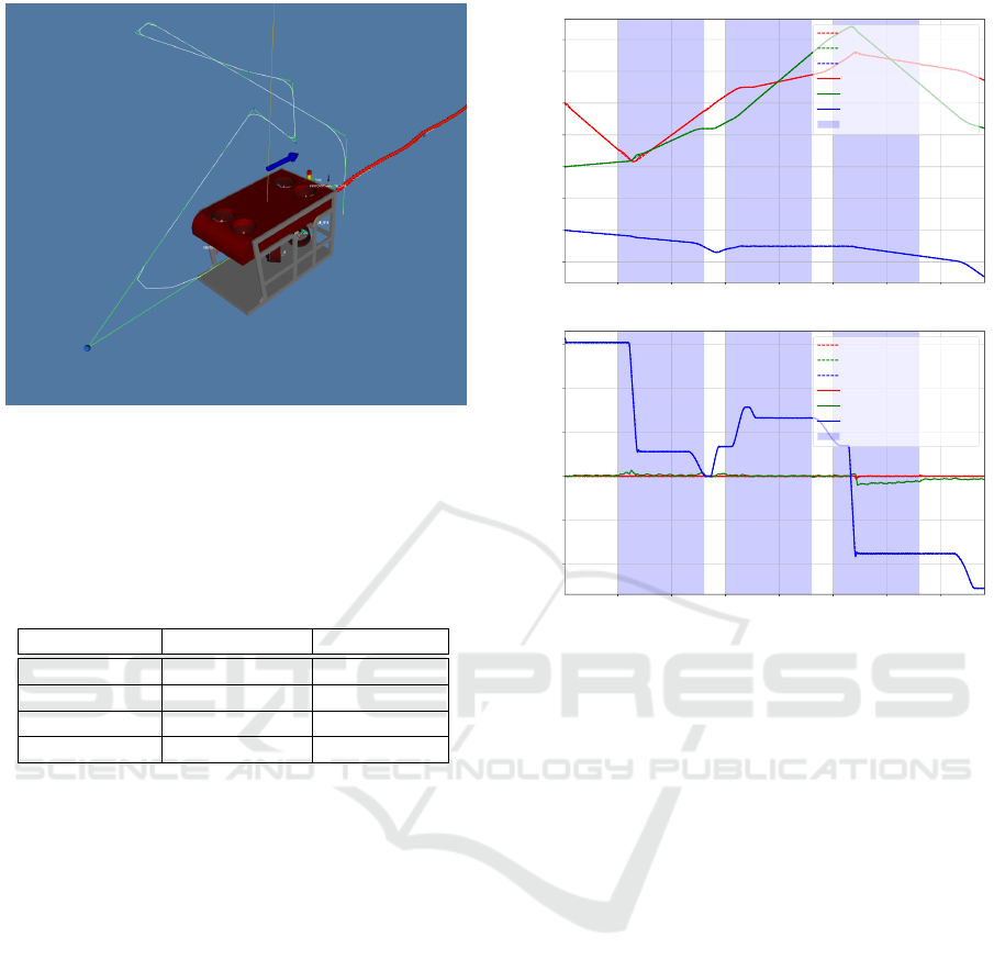
Figure 15: View of the RViz display during the waypoint

following scenario. The green path shows the lines con-

necting the waypoint sequence, the white path represents

the result of the path interpolation with polynomial blends,

the blue arrow shows the direction of the current velocity

vector and the blue spheres represent the waypoints.

Table 10: Comparison of performance metrics using the

new disturbance setup for the waypoint following scenario.

Metric Sliding Mode MIMO PID

RMSE

[m] 0.154 0.059

RMSE

[rad] 0.007 0.005

RMSE

[rad] 0.069 0.036

RMSE

[rad] 0.010 0.006

it might lead to high deviations or unstable results un-

der certain environmental conditions and unmodeled

model uncertainties considering that it is not inher-

ently robust. The optimization of these control strate-

gies using scenarios where the disturbances models

tend to reproduce worst-case examples of possible

perturbations that could occur will help to gain cer-

tainty on the capability of the control algorithm to be

deployed with a speciﬁc vehicle before going to ﬁeld

tests with the real system. More extensive tests, such

as sensitivity analysis against a range of disturbances,

can also be employed to gain more information on the

safe operational limits of the closed-loop system and

will be a subject of future research.

7 CONCLUSIONS

This paper explores the advantages of a methodical

simulation-based controller setup based on its perfor-

mance evaluation. The optimization takes into ac-

count a weighted sum of performance metrics from

the simulated scenario and can be setup to also con-

25 50 75 100 125 150 175

Time [s]

−30

−20

−10

Position [m]

Position

Current disturbance activated

25 50 75 100 125 150 175

Time [s]

−2

−1

Angles [rad]

Orientation

Current disturbance activated

Figure 16: Reference and actual trajectories using the inter-

polated waypoint set for the model-free sliding mode con-

troller.

sider possible disturbances that could occur during the

mission. The performance analysis can also be further

extended, e.g. considering the control efforts and ve-

locity errors.

This framework is facilitated by the modular

structure of the simulation environment used based on

ROS and Gazebo. Its structure allows the combina-

tion of different vehicles, controller, trajectory gener-

ators and disturbance models, that combined with a

task scheduler can be easily initialized with the dif-

ferent conﬁguration parameters by, in this case, by

an optimization process, allowing a high level of au-

tomation of the parameter search method.

After the optimal setup of the two controllers in

the use case presented, a numerical comparison be-

tween their performances can be fairly evaluated un-

der the same conditions, an aspect that can highly

beneﬁt the mission planning phases. This framework

will be further developed to consider model-based

controllers and a benchmarking procedure to be used

on the mission planning for different vehicles and sce-

narios, also focusing on energy consumption and mis-

sion time along with other sources of perturbation,

such as thruster failure and model mismatch, and ex-

tending the validation process to the real underwater

vehicle.

Framework for Fair Comparisons of Underwater Vehicle Controllers - Showcasing the Robustness Properties of a Model-free Sliding Mode

Controller Tuned with a Random-forest-based Bayesian Optimization Approach

111

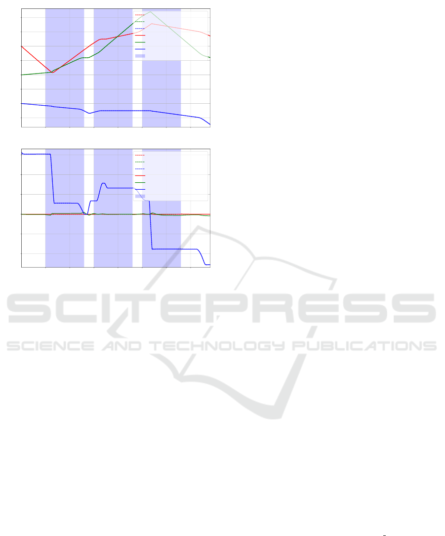
25 50 75 100 125 150 175

Time [s]

−30

−20

−10

Position [m]

Position

Current disturbance activated

25 50 75 100 125 150 175

Time [s]

−2

−1

Angles [rad]

Orientation

Current disturbance activated

Figure 17: Comparison of results for the trajectory tracking

from an interpolated waypoint set for the sliding mode and

PID controllers.

ACKNOWLEDGEMENTS

The work in this paper has been developed as part

of the work undertaken for the EU-funded SWARMs

(Smart and Networking Underwater Robots in Co-

operation Meshes) research project (ECSEL project

number 662107).

REFERENCES

Antonelli, G. (2014). Underwater Robots. Springer Inter-

national Publishing.

Berg, V. (2012). Development and commissioning of a DP

system for ROV SF 30k. Master’s thesis, Institutt for

marin teknikk, NTNU.

Berkenkamp, F., Schoellig, A. P., and Krause, A. (2016).

Safe controller optimization for quadrotors with gaus-

sian processes. In 2016 IEEE International Confer-

ence on Robotics and Automation (ICRA). Institute of

Electrical and Electronics Engineers (IEEE).

Brochu, E., Cora, V. M., and de Freitas, N. (2010). A tuto-

rial on Bayesian optimization of expensive cost func-

tions, with application to active user modeling and hi-

erarchical reinforcement learning. Technical report,

arXiv.org.

Calandra, R., Gopalan, N., Seyfarth, A., Peters, J., and

Deisenroth, M. P. (2014). Bayesian gait optimization

for bipedal locomotion. In Lecture Notes in Computer

Science, pages 274–290. Springer Nature.

Fossen, T. I. (2011). Handbook of Marine Craft Hydrody-

namics and Motion Control. Wiley-Blackwell.

Garc

ıa-Valdovinos, L. G., Salgado-Jim

enez, T., Bandala-

anchez, M., Nava-Balanzar, L., Hern

andez-

Alvarado, R., and Cruz-Ledesma, J. A. (2014).

Modelling, design and robust control of a remotely

operated underwater vehicle. International Journal of

Advanced Robotic Systems, 11(1):1.

Garcia-Valdovinos, L. G., Salgado-Jimenez, T., and Torres-

Rodriguez, H. (2009). Model-free high order sliding

mode control for ROV: Station-keeping approach. In

OCEANS 2009, MTS/IEEE Biloxi-Marine Technology

for Our Future: Global and Local Challenges, pages

1–7. IEEE.

Heise, C. D., Leitao, M., and Holzapfel, F. (2013). Perfor-

mance and robustness metrics for adaptive ﬂight con-

trol - available approaches. In AIAA Guidance, Navi-

gation, and Control (GNC) Conference. American In-

stitute of Aeronautics and Astronautics (AIAA).

Hosseini, M. and Seyedtabaii, S. (2016). Robust ROV path

following considering disturbance and measurement

error using data fusion. Applied Ocean Research,

54:67–72.

Hutter, F., Hoos, H. H., and Leyton-Brown, K. (2011). Se-

quential model-based optimization for general algo-

rithm conﬁguration. In Lecture Notes in Computer

Science, pages 507–523. Springer Nature.

Khadhraoui, A., Beji, L., Otmane, S., and Abichou, A.

(2014). Observer-based controller design for remotely

operated vehicle ROV. In Proceedings of the 11th In-

ternational Conference on Informatics in Control, Au-

tomation and Robotics. Scitepress.

Koenig, N. and Howard, A. (2004). Design and use

paradigms for Gazebo, an open-source multi-robot

simulator. In 2004 IEEE/RSJ International Confer-

ence on Intelligent Robots and Systems (IROS) (IEEE

Cat. No.04CH37566). Institute of Electrical and Elec-

tronics Engineers (IEEE).

Lantos, B. and M

arton, L. (2011). Nonlinear Control of

Vehicles and Robots. Springer London.

Lindauer, M., Eggensperger, K., Feurer, M., Falkner,

S., Biedenkapp, A., and Hutter, F. (2017).

SMAC v3: Algorithm Conﬁguration in Python.

https://github.com/automl/SMAC3.

Manh

aes, M. M. M., Scherer, S. A., and Douat,

L. R. (2016a). Unmanned Underwater Ve-

hicle (UUV) Simulation Package for Gazebo.

https://github.com/uuvsimulator/uuv simulator.

Manh

aes, M. M. M., Scherer, S. A., Voss, M., Douat,

L. R., and Rauschenbach, T. (2016b). UUV simu-

lator: A Gazebo-based package for underwater inter-

vention and multi-robot simulation. In OCEANS 2016

MTS/IEEE Monterey. Institute of Electrical and Elec-

tronics Engineers (IEEE).

Molero, A., Dunia, R., Cappelletto, J., and Fernandez, G.

(2011). Model predictive control of remotely operated

SIMULTECH 2017 - 7th International Conference on Simulation and Modeling Methodologies, Technologies and Applications

112

underwater vehicles. In IEEE Conference on Decision

and Control and European Control Conference. Insti-

tute of Electrical and Electronics Engineers (IEEE).

Parra-Vega, V. and Arimoto, S. (1995). Adaptive control for

robot manipulators with sliding mode error coordinate

system: free and constrained motions. In Proceedings

of 1995 IEEE International Conference on Robotics

and Automation. Institute of Electrical and Electronics

Engineers (IEEE).

Parra-Vega, V., Arimoto, S., Liu, Y.-H., Hirzinger, G., and

Akella, P. (2003). Dynamic sliding PID control for

tracking of robot manipulators: theory and experi-

ments. IEEE Transactions on Robotics and Automa-

tion, 19(6):967–976.

Soylu, S., Proctor, A. A., Podhorodeski, R. P., Bradley, C.,

and Buckham, B. J. (2016). Precise trajectory con-

trol for an inspection class ROV. Ocean Engineering,

111:508–523.

Stepanyan, V., Krishnakumar, K., Nguyen, N., and Eykeren,

L. V. (2009). Stability and performance metrics for

adaptive ﬂight control. In AIAA Guidance, Naviga-

tion, and Control Conference. American Institute of

Aeronautics and Astronautics (AIAA).

Zhu, K. and Gu, L. (2011). A MIMO nonlinear robust con-

troller for work-class ROVs positioning and trajectory

tracking control. In 2011 Chinese Control and Deci-

sion Conference (CCDC). Institute of Electrical and

Electronics Engineers (IEEE).

Framework for Fair Comparisons of Underwater Vehicle Controllers - Showcasing the Robustness Properties of a Model-free Sliding Mode

Controller Tuned with a Random-forest-based Bayesian Optimization Approach

113