Plane Equation Features in Depth Sensor Tracking

Mika Taskinen, Tero S

antti and Teijo Lehtonen

University of Turku, Department of Future Technologies, 20014 Turun Yliopisto, Finland

Keywords:

Depth, Sensor, Plane, Equation, Tracking, 3D, Augmented Reality.

Abstract:

The emergence of depth sensors has made it possible to track not only monocular cues but also the actual

depth values of the environment. This is especially useful in augmented reality solutions, where the position

and orientation (pose) of the observer need to be accurately determined. Depth sensors have usually been used

in augmented reality as mesh builders and in some cases as feature extractors for tracking. These methods

are usually extensive and designed to operate by itself or in cooperation with other methods. We propose a

systematic light-weight algorithm to supplement other mechanisms and we test it against a random algorithm

and ground truth.

1 INTRODUCTION

Today the use of augmented reality solutions is in-

creasing and more efﬁcient methods for tracking are

being developed for motion sensors and conventional

cameras. Using depth sensors in this manner is a

fairly new area, in comparison as they have not been

accurate or mobile enough to be used in augmented

reality. Over the last few years this has changed dras-

tically and now some algorithms and methods have

ﬁnally been researched for the depth sensors.

All sensors have their faults when tracking the

pose. A conventional camera might lose its track

when the captured image lacks details. Motion sensor

has to be accurate and record data in high frequency.

Even then the pose might drift unless corrected with

other methods. A depth sensor usually does not work

under sunlight conditions or when the distance to the

tracked surroundings is too great. These, and possibly

other methods, need to be combined to achieve more

robust tracking.

The advantage of depth sensors in tracking is the

actual depth data which contains real distances to tar-

get areas. These distances can be used to isolate ba-

sic formations like planes, cubes and spheres. The

data can also be used when building up a more robust

model of the surroundings.

Currently the depth sensors are mostly used to

map the surroundings of the user and tracking is usu-

ally done by a combination of motion sensors, con-

ventional cameras and location services. Some tools

for depth tracking exist, but as of yet, their usage has

been limited. As a scanning feature, Microsoft has

introduced KinectFusion to be used with Kinect to

scan objects with limited space requirements and lim-

ited depth tracking abilities (Newcombe et al., 2011).

A plane ﬁltering method with Ransac (random) fea-

ture selection system has been suggested to fully im-

plement depth sensor tracking (Biswas and Veloso,

2012).

Due to the current limitations of the depth sen-

sors in range and accuracy, a lighter and more sys-

tematic feature and tracking algorithm is proposed to

support other tracking mechanisms. By keeping fea-

tures as plane equations, no real edges and corners are

detected, only intersections between inﬁnite planes.

This makes the algorithm much faster than an algo-

rithm that uses computing power to detect physical

edges. Systematic detection makes plane equation

tracking a more adjustable tool while giving possibil-

ity to increase robustness. Changing the grid size can

be done on the ﬂy, and it provides an easy tradeoff

between execution time and accuracy.

The paper is organized as follows: The paper be-

gins with introduction where we lead the reader into

the subject by presenting the problem. Next section,

Related Work, gathers references to other papers and

methods to explain the current state of the develop-

ment. The Plane Equation Detection section intro-

duces the solution (algorithm) with operation ﬂow

and equations describing the entire method step-by-

step. We have tested our process against another one

Taskinen, M., Säntti, T. and Lehtonen, T.

Plane Equation Features in Depth Sensor Tracking.

DOI: 10.5220/0006425700170024

In Proceedings of the 14th International Joint Conference on e-Business and Telecommunications (ICETE 2017) - Volume 5: SIGMAP, pages 17-24

ISBN: 978-989-758-260-8

and show the technical readings in depth in Results.

The Discussion section covers additional ideas, like

tracking, to further develop the solution. The ﬁnal

section, Conclusions, summarizes the paper and the

results overall.

2 RELATED WORK

The plane equation method is not the ﬁrst idea involv-

ing depth sensors and tracking since the sensors have

become consumer products. Other propositions have

been made to be used for either feature extraction or

to gather data. Here are a few of those ideas:

In a paper (Ataer-Cansizoglu et al., 2013), track-

ing is done by extracting points and planes from depth

data and an extended prediction algorithm is used.

The paper does not include details on how the actual

feature detection is accomplished.

The paper (Fallon et al., 2012), introduces Kinect

Monte Carlo Localization (KMCL) to calculate pose

from point cloud provided by a depth sensor. KMCL

uses a 3D-map of the surroundings and uses simulated

depth and color images as a comparison. The KMCL

requires a model of the tracked environment which

differentiates it from the proposed method.

For a more detailed information on different meth-

ods, please see (Taskinen et al., 2015), a literature re-

view on different depth related tracking methods in

augmented reality. The report lists a total of 21 depth

sensor related tracking and scanning articles and cat-

egorizes them by their main purpose: Localization,

reconstruction or both.

2.1 Plane Filtering

Plane ﬁltering is a way to make the tremendous

amount of data a depth sensor produces a little eas-

ier to handle in computational sense. Any pixel-by-

pixel method becomes very unusable when the accu-

racy of one pixel can vary between 1 mm to 30 mm.

The problem is compounded by the fact that the data

is most likely handled in 3D-coordinates. To counter

this problem, the data needs to be handled in larger

groups, hence the plane ﬁltering.

The base idea is to take only a few points (sam-

ples) from data and derive possible planes from them.

To actually use these planes in mesh building and

tracking, a further edge detection step must be per-

formed.

In the article (Biswas and Veloso, 2012) a Ransac

based plane ﬁltering system is proposed. In short, the

plane detection is done by randomly selecting sample

points to form planes and then continuing on, again

randomly, to extend that plane with additional sam-

ples. Our approach improves stability in cases where

random sampling may result in unpredictable data

loss. Additionally, our approach is conﬁgurable dur-

ing run time, allowing a clear tradeoff between exe-

cution time and accuracy. Random selection can be

tuned in similar fashion, but the resulting behaviour

is not so easily predictable. One set of random points

can generate more than satisfactory results for a single

run, but on the next run the same number of random

points can yield sub-par results. With our approach

the results show a constant quality level for each grid

size. This allows the ﬁne tuning to be performed in a

predictable fashion.

2.2 Simultaneous Localization and

Mapping

Simultaneous Localization And Mapping (SLAM)

has been originally developed for conventional color

cameras but the idea can be processed with depth sen-

sors also (Riisgaard and Blas, 2005). Closest prac-

tical example of depth SLAM would be KinectFu-

sion (Newcombe et al., 2011), where depth sensor is

used to map the data and aid the tracking in visually

obscure situations like in dark spaces or colorless en-

vironments.

Real-Time mapping in SLAM has always been a

problem in computer power and memory use, and in

KinectFusion case the mapped model is in a memory

limited cube of voxels. Other solutions have solved

the memory issue by limiting the quality of the map

or by using extensions to memory that may slow the

computation (Whelan et al., 2012).

The part of the SLAM our method uses, does not

require as much detail. This keeps the computation

and memory consumption at a lower level, so it will

not be an issue (See Section 5).

3 PLANE EQUATION

DETECTION

This paper introduces a new method to be used with

depth data to cover all the applications using multi-

ple tracking methods with limited computing power.

In terms of computing power, the plane equations are

relatively easy to calculate.

Detecting planes in a depth image is simple when

the right mathematical tools are being used. The three

states of the proposed plane detection are illustrated

in Figure 1. By using a split grid over the image, the

detection task can be quantiﬁed into smaller tasks. In

SIGMAP 2017 - 14th International Conference on Signal Processing and Multimedia Applications

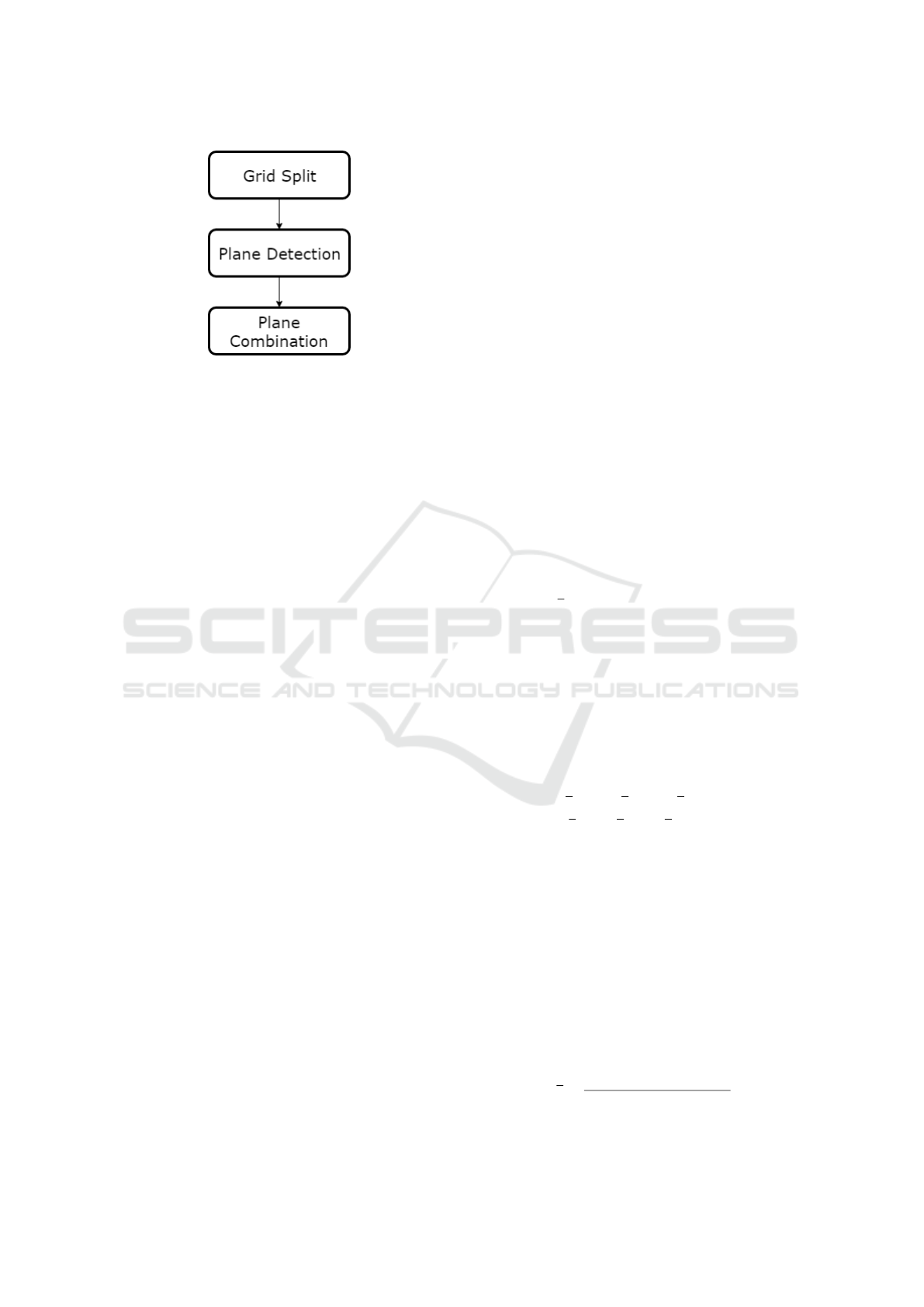
Figure 1: The three states of plane detection.

short, the grid cells will be tested for planes by using

three corner points as a plane deﬁnition. The fourth

corner point will then be used as a veriﬁer for that

cell. If the fourth corner point belongs to the plane,

the entire cell is a plane and can be used further. It is

worth noting, that it is possible to make the detection

more robust by using more points in the cell to verify

the plane. However, such a mechanism has not been

implemented for this paper, and it remains as future

work for later.

The next phase is to combine these cell planes into

a larger whole. This is done by comparing cells by us-

ing the direction (normal) of the plane and one point

from each plane. If they match, within an acceptable

error, they will be combined into one larger plane.

This task will be repeated over all the cells that have

been detected as planes.

The ﬁnal task is to ﬁlter useless information. All

the planes that do not contain enough cell planes will

be removed. For instance the corners of a room can

cause plane-like data points, when the left side of the

grid hits one wall, and the right side hits the other

wall. Situations like this are ﬁltered out simply by

requiring that a plane must have enough supporting

cells to be accepted.

Figure 2 shows the method in use. The photo is

taken from a laboratory room to demonstrate the ef-

fectiveness of the algorithm in an environment where

there are a lot of obstructing objects. Planes detected

are named and then colored according to direction

they are facing. As can be seen, planes are detected

even when there are other objects creating distrac-

tions.

3.1 Notable Difference

Plane Equation Detection differs from any other tech-

nique mostly by detecting ”inﬁnite” planes. This

mechanism does not directly detect physical edges of

the planes as the method is mainly intended to pro-

duce features for tracking. Edges and corners can

still be detected mathematically by using plane inter-

sections or physically by doing edge search after the

equation has been found.

In Figure 2, the planes are inﬁnite but the visi-

ble edge is a border of the group of grid cells that

form a plane. This border can also be used to map

the real edges when needed. Mathematically calcu-

lated edges and corners are actually used in tracking

when the orientation needs to be more robust or the

location needs to be tracked. The mathematical in-

tersections provide more accuracy and stability than

directly detected corners because the calculations use

several points instead of just the corner. This averages

out much of the noise which would affect the direct

detection with full effect.

3.2 Mathematical Functions

This part describes all the mathematical functions in-

volved in plane detection.

3.2.1 Deﬁnition of Plane

The simplest way to describe a plane is with it’s nor-

mal vector (v) and one contained point (p) as illus-

trated in Figure 3. This plane can be transformed into

linear function by using Equation 1. Planes can also

be deﬁned with two vectors instead of a normal vec-

tor. These vectors are parallel with the plane and di-

vergent with each other. With two scalars multiplied

with these vectors, any position in the plane can be

generated. In this way, the calculation of plane func-

tion is faster but intersection and inclusion calcula-

tions are slower.

∗ p

+ v

∗ p

+ v

∗ p

−

∗ x + v

∗ y + v

∗ z) = 0

(1)

3.2.2 Plane from Three Points

A plane needs to be deﬁned using three points of a

cell rectangle. The point contained by the plane can

be any of the given three points (p

, p

) and the

direction is calculated by cross product calculation us-

ing Equation 2. If using two direction vectors is pre-

ferred, then a simple subtraction between the points

will sufﬁce (calculation without the cross product).

For this paper the cross product has been chosen, be-

cause it will be beneﬁcial in the following step.

v =

((p

− p

) × (p

− p

))

||p

− p

|| ∗ ||p

− p

(2)

Plane Equation Features in Depth Sensor Tracking

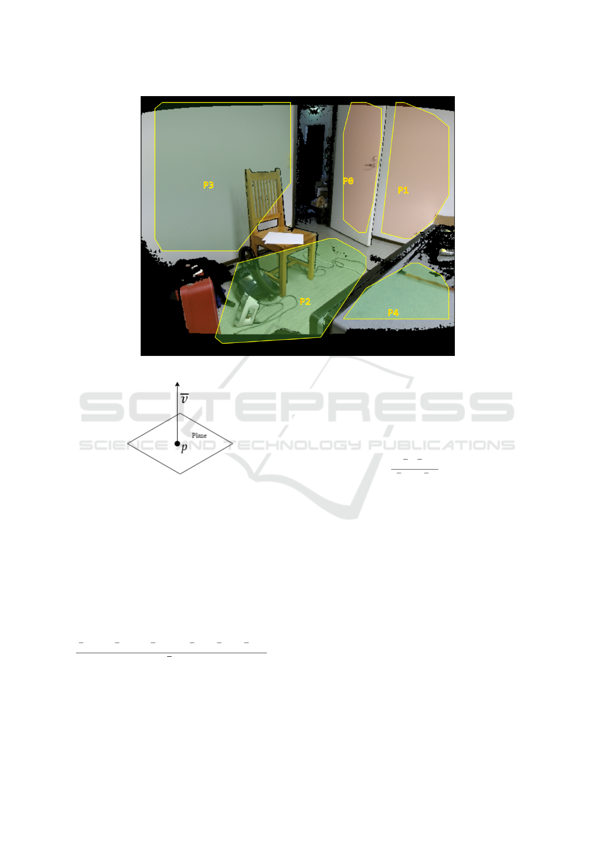
Figure 2: An image of real time feature extraction with Microsoft Kinect 2.

Figure 3: The deﬁnition of plane.

3.2.3 Point in Plane

Point in plane equation is used for detecting if the ear-

lier mentioned fourth point is part of the newly de-

ﬁned cell plane. It is also used in plane similarity

comparison in the next phase. The Equation 3, which

is based on Equation 1, is used for this. This calcu-

lation requires the normal vector. When the direction

vectors are being used, a cross product must be cal-

culated to get the normal. If the cross product was

already calculated in the previous step, it can be used

directly without additional computations.

∗ p

+ v

∗ p

+ v

∗ p

− (v ∗ x + v ∗ y + v ∗ z)|

||v||

≤ θ

(3)

In Equation 3, the θ is a threshold minimum dis-

tance of the point from the plane and it makes the

equation usable with imperfect values the depth im-

age displays.

3.2.4 Comparing Vector Direction

In order to ﬁnd out, if two planes are similar, we must

check if the planes have a unifying point and are fac-

ing the same direction. For the direction, a dot prod-

uct is used according to Equation 4.

1 −

· v

||v

|| ∗ ||v

≤ θ (4)

4 RESULTS

One way to understand the beneﬁts of the systematic

plane equation detection is to compare it with a ran-

dom detection method. It does not matter what kind of

random mechanism is used, as the point is to show the

unreliability of any random method. In this case, the

random method does predetermined amount of ran-

dom hits in the image and then tries to hit three more

times around the original point to get the four points

necessary to test for a plane equation. The rest of the

process is equivalent to the proposed plane equation

method.

Another way to compare the methods is a timed

benchmark where computation times are compared

with different parameters. As the comparison is done

between systematic and random algorithms, the re-

sults are not exact. To evaluate any random method,

an iteration of many attempts is required and these

SIGMAP 2017 - 14th International Conference on Signal Processing and Multimedia Applications

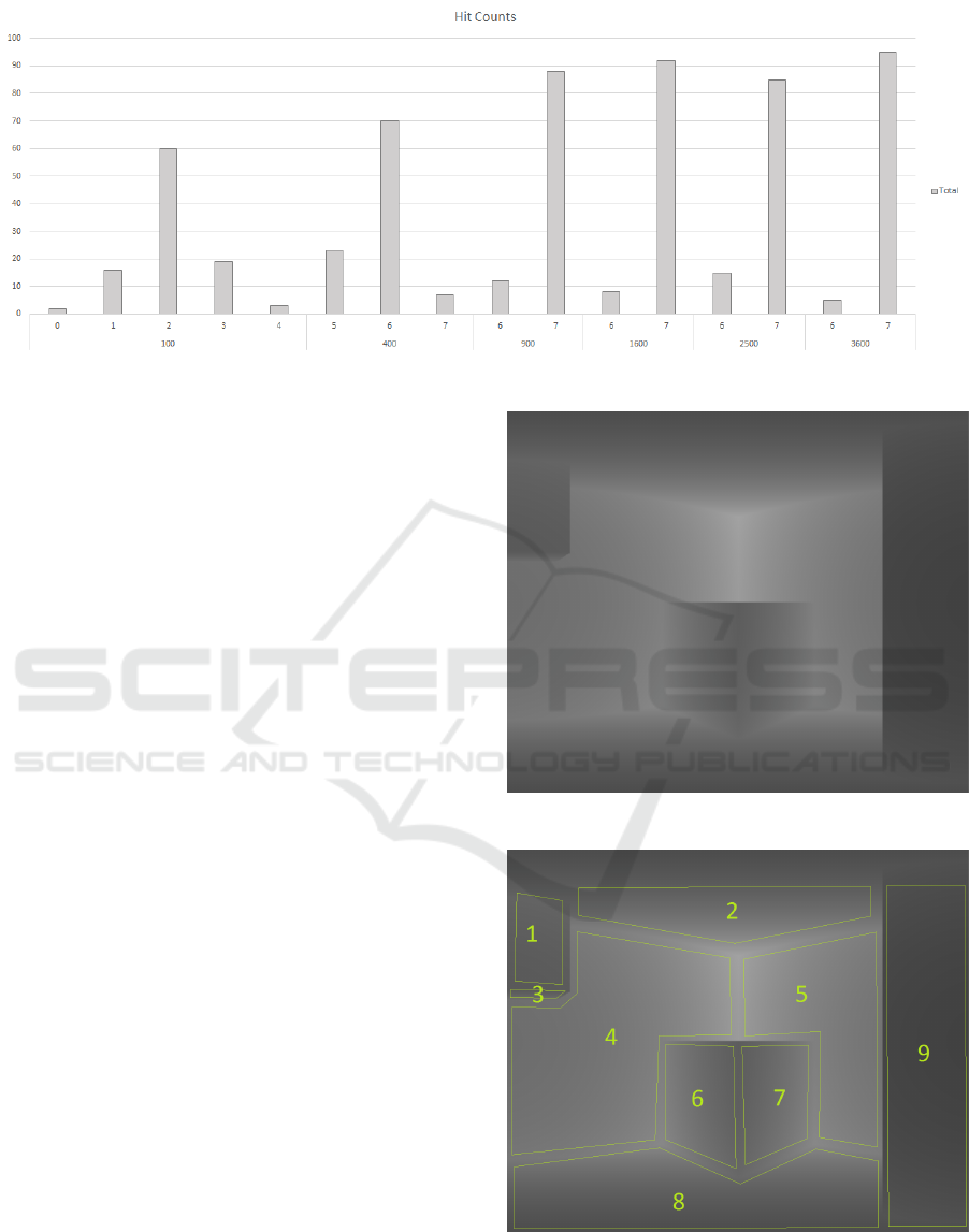
Figure 4: Distribution of plane counts for different random iteration counts.

kind of loops may be optimized at compilation or

processing. Thus, unpredictable effects may occur.

Therefore, the timed benchmark is still required to see

if the methods are even in the same level.

Both algorithms are tested using computer gener-

ated virtual depth data illustrated in Figures 5 and 6.

This provides a stable and consistent reference, un-

like the real world data from a noisy sensor, which

would be slightly different for each run even in the

same location. Also the ground truth is known and

readily available, while real world data would have to

be evaluated by a human to obtain the correct value

for each frame. The Figure 6 shows how many planes

are detected with naked eye.

The tests have a number of parameters affecting

them with similar and dissimilar parameters for each

algorithm. Most of these parameters are chosen so

that they produce the best possible result for both al-

gorithms. These parameters are shown in Table 1.

Field of View and Image Resolution are both based on

Kinect speciﬁcations. The iterations are selected to

create balance between probability testing and com-

puting time as doing more iterations take more time

and doing less result in less accurate data. The other

parameter values are selected based on experiencing.

Both algorithms have one changing variable used

in benchmark. For the systematic method it is the grid

division and for the random method it is the point

count per iteration. Figures 9 and 7 show the used

values for these variables in the x-axis (for instance

40x40=1600 means 40 by 40 grid division for the sys-

tematic algorithm and 1600 points for the random al-

gorithm). The iteration goes through same amount of

plane equation tests between algorithms in each case.

The Figure 7 shows the amount of detected planes

for both algorithms and also has the ground truth

count for reference. The random method produces a

variety of results over many iterations and the one se-

Figure 5: Depth image of ground truth.

Figure 6: Ground truth with visually detected planes.

lected for Figure 7 is the most probable one selected

from the overall test results shown in Figure 4. As

seen in Figure 4, the results can vary when random

Plane Equation Features in Depth Sensor Tracking

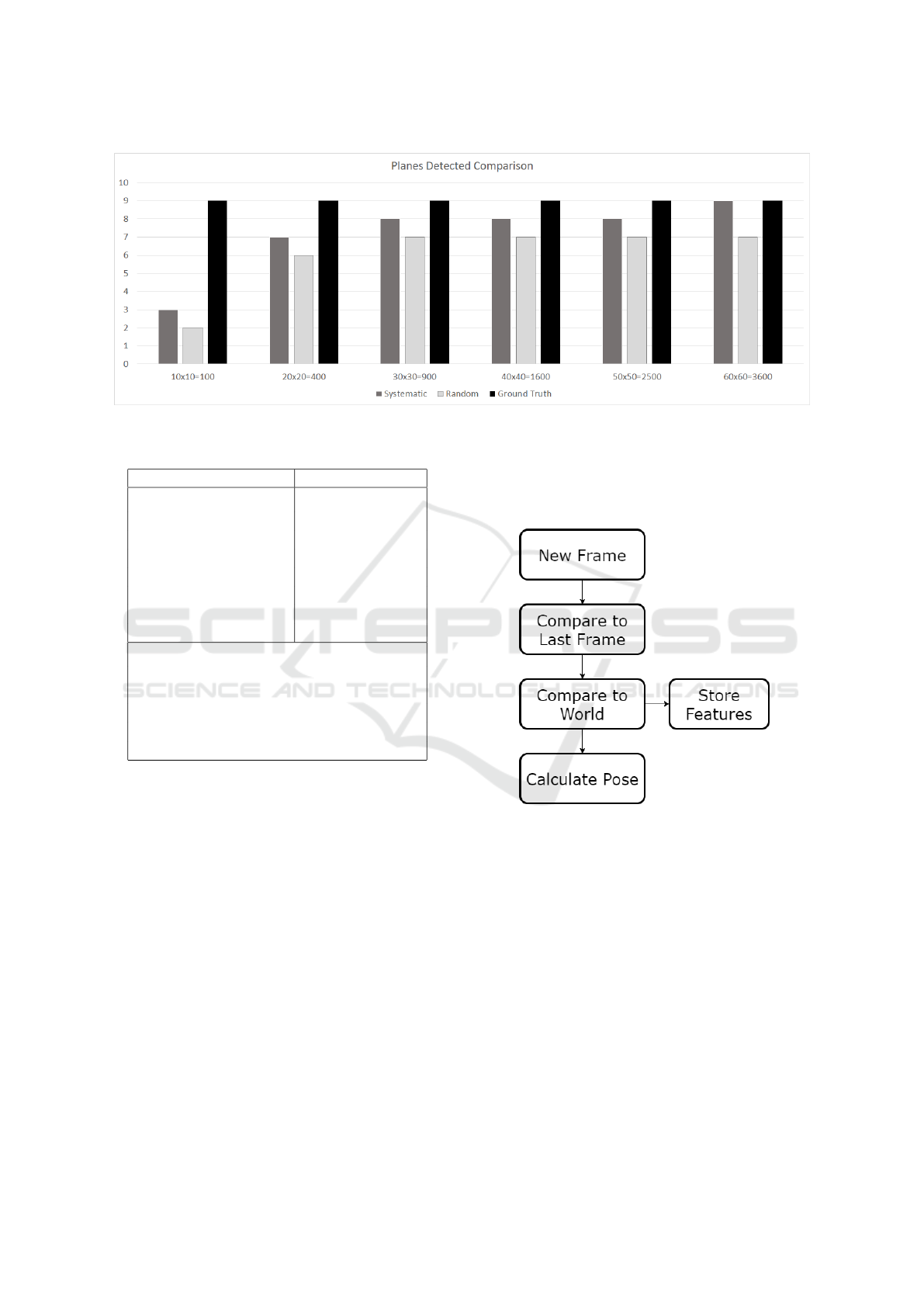
Figure 7: Comparison between random and systematic detection in detected plane count with ground truth.

Table 1: The constant parameters for benchmark.

Parameter Value

Field of View

100

◦

Image Resolution

512 x 424

Iterations

100

Maximum Radius

Minimum Plane Count

Minimum Radius

Normal Epsilon

0,1

Point Epsilon

0,3 [m]

A parameter of depth image.

Iteration count for random algorithm.

Distance variable for random point hits.

Required number of planes in combination stage.

Allowed error for direction comparison.

Allowed error for point-in-plane test.

selection is being used, but as the number of iteration

cycles grows, the count points more heavily towards

one value.

The timed benchmark shown in Figure 9 leans

strongly in favour of random detection. The differ-

ence in elapsed time between both methods is consid-

erable but unreliable. Since the algorithms are not op-

timized, the optimizations in the compilation and pro-

cessing phase introduce unpredictable effects to the

simulation. Thus, observer affects the observed.

5 DISCUSSION

After optimization, the feature extraction can produce

reliable timed benchmark results. In different stages

of development, the algorithm has performed differ-

ently and in some cases could even perform fast us-

ing high quality settings (60x60 grid division). Later

modiﬁcations made the library more generic and reli-

able in plane detection but slowed down the process.

Therefore, better performance can be expected.

Figure 8: The ﬂow of the tracking part.

The subject of the paper covers features for track-

ing but not the tracking itself. In this section we in-

troduce an idea for tracking that can be implemented

with plane equation features. The phases of the track-

ing are shown in Figure 8. Tracking with plane equa-

tions begins with comparing two consecutive image

frames. To make the algorithm faster we can assume

that the sensor won’t move much between frames.

That way the planes that were detected in the last

frame are relatively close to the new ones. Planes

that have ”wandered” far can then be detected as new

planes unless the entire frame has shifted to a new po-

sition. In this case we need to match at least a few

combinations to get the best result of our new orien-

tation and position (pose). We can do a fast detection

run by ﬁnding the closest planes and then check them

SIGMAP 2017 - 14th International Conference on Signal Processing and Multimedia Applications

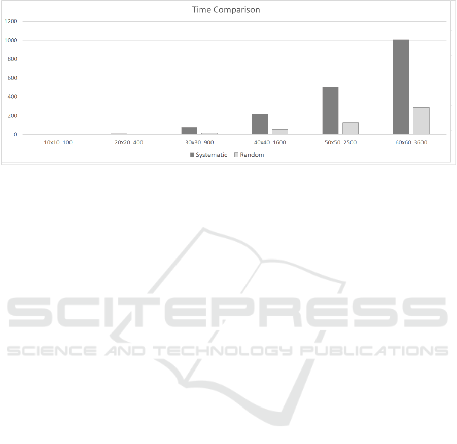
Figure 9: Comparison of execution times between random and systematic detection.

by comparing the translation values (initial guess).

When the plane matching has been done and the

pose translation has been found, we can start match-

ing our new frame with a world of planes. A world

of planes is our global storage of every plane detected

so far and can be used in the detection throughout the

entire tracking session. Some new planes, detected

between frames, might have been detected already in

some earlier frame and have more precise information

on pose and can aid in tracking. Constant adjustment

of global plane collection is required.

6 CONCLUSIONS

We have shown that our plane detection algorithm is

more reliable than random detection when detecting

planes. By increasing quality (grid division), the al-

gorithm quickly approaches the ground truth plane

count. This is useful for a support algorithm as we

can have desired output with low level computation.

When enough planes have been detected, the informa-

tion is sufﬁcient to conﬁrm the pose the other tracking

methods have calculated.

Actual depth image is noisy and in consecutive

frames there are differences in almost every pixel. In

every feature extraction method, this problem is ad-

dressed by using strong features that are either an av-

erage of smaller components or have something very

deﬁning in them. Combining the data into larger

planes does the same in plane equation detection, pro-

viding good tolerance towards sensor noise at a low

computational effort.

ACKNOWLEDGEMENTS

The research has been carried out during the

MARIN2 project (Mobile Mixed Reality Applica-

tions for Professional Use) funded by Tekes (The

Finnish Funding Agency for Innovation) in collabo-

ration with partners; Defour, Destia, Granlund, In-

frakit, Integration House, Lloyd’s Register, Nextfour

Group, Meyer Turku, BuildingSMART Finland, Ma-

chine Technology Center Turku and Turku Science

Park. The authors are from University of Turku, Fin-

land.

REFERENCES

Ataer-Cansizoglu, E., Taguchi, Y., Ramalingam, S., and

Garaas, T. (2013). Tracking an RGB-D camera using

points and planes. Proceedings of the IEEE Interna-

tional Conference on Computer Vision, pages 51–58.

Biswas, J. and Veloso, M. (2012). Planar polygon extraction

and merging from depth images. IEEE International

Conference on Intelligent Robots and Systems, pages

3859–3864.

Fallon, M. F., Johannsson, H., and Leonard, J. J. (2012).

Efﬁcient scene simulation for robust monte carlo lo-

calization using an RGB-D camera. Proceedings -

IEEE International Conference on Robotics and Au-

tomation, pages 1663–1670.

Newcombe, R. a., Izadi, S., Hilliges, D., Molyneaux, D.,

Kim, D., Davison, A. J., Kohi, P., Shotton, J., Hodges,

S., and Fitzgibbon, A. (2011). KinectFusion : Real-

Time Dense Surface Mapping and Tracking. IEEE In-

ternational Symposium on Mixed and Augmented Re-

ality, pages 127–136.

Riisgaard, S. and Blas, R. (2005). Slam for dummies.

Taskinen, M., Lahdenoja, O., S

antti, T., Jokela, S., and

Lehtonen, T. (2015). Depth Sensors in Augmented

Reality Solution - Literature Review.

Plane Equation Features in Depth Sensor Tracking

Whelan, T., Johannsson, H., Kaess, M., Leonard, J. J., and

Mcdonald, J. (2012). Robust Tracking for Real-Time

Dense RGB-D Mapping with Kintinuous. RSS Work-

shop on RGB-D: Advanced Reasoning with Depth

Cameras, page 10.

SIGMAP 2017 - 14th International Conference on Signal Processing and Multimedia Applications