A Solution for Ice Accretion Detection on Wind Turbine Blades

Jocelyn Sabatier

, Patrick Lanusse

, Benjamim Feytout

and Serge Gracia

Bordeaux University, IMS Lab., UMR 5218 CNRS, 351 Cours de la Libération, 33405 Talence, France

Bordeaux INP, IMS Lab., UMR 5218 CNRS, 351 Cours de la Libération, 33405 Talence, France

VALEOL, Parc de l’Intelligence Environnementale, 213 Cours Victor Hugo, 33323 Bègles Cedex, France

Keywords: Wind Turbine, Blade Ice Detection, Observer, Anti-icing Device.

Abstract: This paper proposes a solution for ice accretion detection on wind turbine blades. The solution involves an

active deicing device that uses a conductive polymer paint to heat relevant surfaces of the blade under

electric potential difference. This deicing system is used here to perform a dynamic thermal characterization

of the blade for various operating conditions (with or without ice, with or without wind). The dynamical

behavior differences highlighted are then exploited using a dynamic observer to detect ice accretion through

the control signal produced by the observer. Tests carried out in a climatic chamber showed the validity and

the accuracy of the proposed method.

1 INTRODUCTION

Cold areas are often attractive regions for wind

turbine installation for two main reasons:

- they are well exposed to wind,

- the low temperatures increase air density, thus

increasing the kinetic energy of the wind and

consequently, the power captured by the wind

turbine.

However, their wind turbine blades are subjected

to icing which can lead to serious consequences for

the production, maintenance and durability of the

whole turbine (Jasinski et al., 1998) (Hochart et al.,

2008).

Ice accretion can be caused by freezing rain,

drizzle, freezing fog, or frost when the wind turbine

is installed near water bodies. It usually appears on

the intrados (to a lesser degree) and extrados, and /

or on the leading and trailing edges (Kraj and

Bibeau, 2010).

Icing reduces the aerodynamic efficiency of the

blades as it changes the blade geometrical profile.

This leads to production losses (Jasinski et al.,

1998), (Ronsten, 2004).

Ice accretion also creates additional and

unbalanced loads that cause increased material

fatigue, leading to premature wear or damage to

major elements of the kinematic chain (impact on

the multiplier and the generator) (Ganander and

Ronsten, 2003) (Frohboese and Anders, 2007) (Virk

et al., 2010). The mass of accumulated ice can

significantly increase vibrations and also the radial

loads on the blades due to centrifugal force. The

system fastening the blades to the hub must be

specifically sized to support the extra stress and

avoid mechanical failure. Such a situation may

require stopping the turbine during severe frost

events.

From a safety point of view, chunks of ice can be

detached during the turbine shutdown or can be

projected during operation, causing lethal risks to

maintenance operators or any other person in the

vicinity of the wind turbine (Seifert, 2003).

Many solutions have been proposed in the

literature to fight against turbine blade ice accretion

(Parent and Ilinca, 2011), such as passive

technologies, which aim to prevent the formation of

ice on the blades (Kimura et al., 2003), (Dalili et al.,

2009), or active technologies which operate when

ice is detected. Most of these technologies come

from the field of aviation and are based on

mechanical deformation or the use of a heater for the

leading edge (Botura and Fisher 2003) (Laakso and

Peltola, 2005).

Active technologies require a means to detect ice

accretion. According to (Homola et al., 2006) and

(Parent and Ilinca, 2011), icing can be detected

either directly or indirectly. Direct methods detect a

change in a physical property caused by ice

414

Sabatier, J., Lanusse, P., Feytout, B. and Gracia, S.

A Solution for Ice Accretion Detection on Wind Turbine Blades.

DOI: 10.5220/0006403904140421

In Proceedings of the 14th International Conference on Informatics in Control, Automation and Robotics (ICINCO 2017) - Volume 1, pages 414-421

ISBN: 978-989-758-263-9

accretion such as (and not cited in (Homola et al.,

2006) (Parent and Ilinca, 2011)) mass (Skrimpas et

al., 2016), reflective properties (Berbyuk et al.,

2014), electrical or thermal conductivity, dielectric

coefficient and inductance (Owusu et al., 2013).

Indirect methods are based upon detecting the

weather conditions that lead to icing (humidity and

temperature).

In this paper, a direct method is proposed. It

involves a de-icing device built by the authors and

recently published (Sabatier et al., 2016). This de-

icing device uses a conductive polymer paint to heat

relevant surfaces of the blade under potential

difference. It is used here to perform a dynamical

thermal characterization of the blade for various

operating conditions (with or without ice, with or

without wind). The dynamical behavior differences

highlighted are then exploited using a dynamic

observer to detect ice accretion through the control

signal produced by the observer.

2 PROTOTYPE AND DEICING

DEVICE PRESENTATION

The proposed ice accretion detection method

involves an active de-icing device recently published

(Sabatier et al., 2016). This de-icing device is based

on heating relevant surfaces of the blade with

conductive polymer paint under electric potential

difference (Rescoll, 2011). Current flow through the

paint film causes heating by the Joule effect that is

proportional, among other things, to the film surface

and thickness. The paint strip power supply is

ensured by electrodes connected to the wind turbine

auxiliaries from the hub.

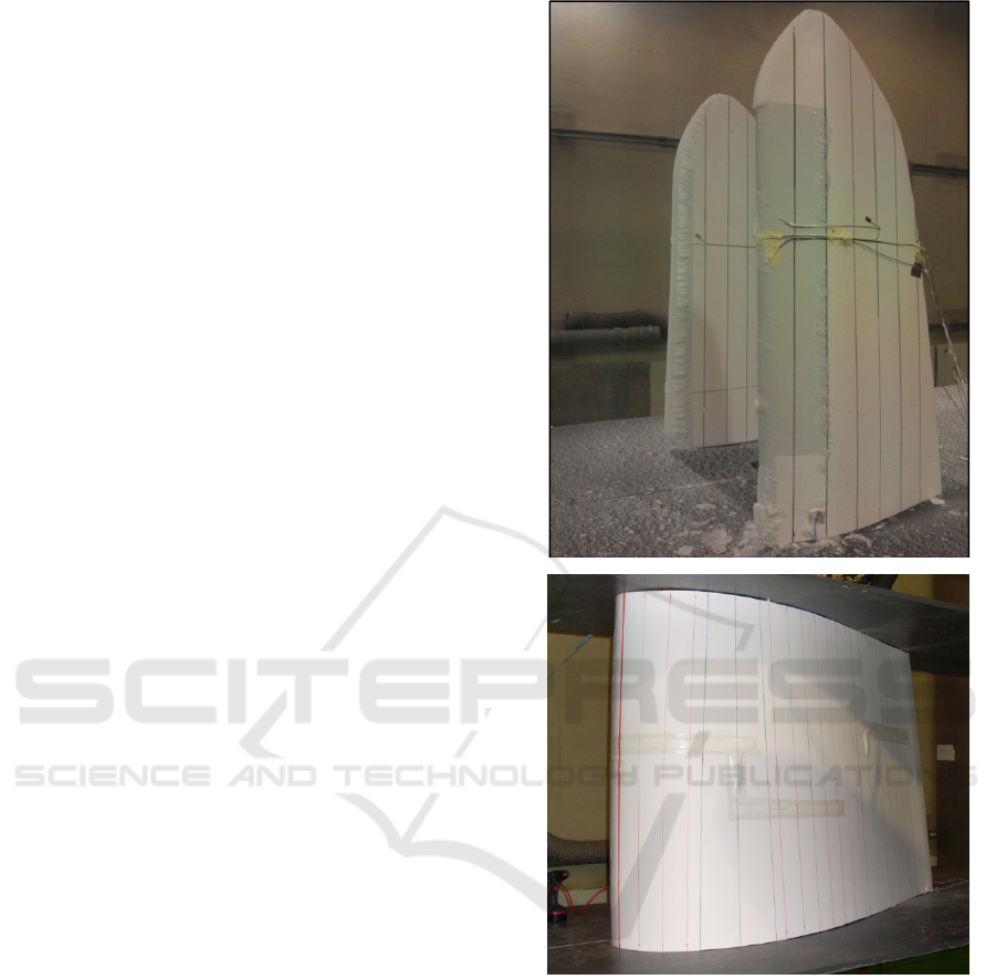
For dynamical modeling and to evaluate the ice

accretion detection method, prototypes of the blade

root and the blade tip were constructed (figure 1).

They integrate different layers of paint (grey parts)

and thermocouples. They were used in a climatic

wind tunnel at the “Centre Scientifique et Technique

du Bâtiment (CSTB)” in Nantes (France) to learn

more about how frost develops on a blade and

especially on what parts of the blade. These

prototypes were also used to obtain a dynamical

model linking the voltage applied on the blade to the

temperature at various points of the paint strips and

also to validate the temperature control system.

Figure 1: Blade tip and blade root prototypes used in the

atmospheric wind tunnel.

3 THERMAL MODELING

3.1 Thermal Model with or without Ice

To obtain a thermal model of the blade heating

system, the simplified representation of figure 2 was

used. It comprises a blade (fiberglass and epoxy

resin) having a large size (in the longitudinal

direction, not shown here) fitted with two electrodes

and then partially covered with paint. A sensor

measures the temperature at the center of the paint

A Solution for Ice Accretion Detection on Wind Turbine Blades

415

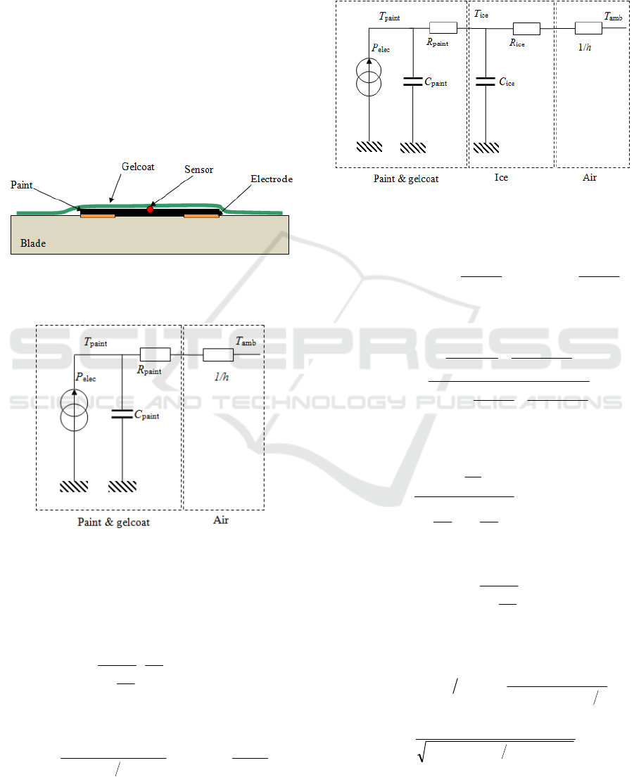
strip. The assembly is protected and separated from

ambient air by a layer of gelcoat.

As shown in (Sabatier et al., 2016), the thermal

resistance and capacity of the blade (epoxy resin)

can be neglected due to the high thermal resistance

value of the blade. Without ice, the resulting

thermal model is thus represented by figure 3, where

paint

and T

amb

are respectively the paint & gelcoat

temperature and the ambient air temperature. R

paint

and C

paint

are respectively the thermal resistance and

capacity of the paint & gelcoat. P

elec

is the thermal

power produced by the paint and h is the paint-air

convection coefficient. In view of the low respective

thicknesses of the paint and the gelcoat, they were

considered as the same material.

Figure 2: Simplified representation (transverse section) of

the blade, the conductive paint, the electrode and the

gelcoat protection.

Figure 3: Simplified thermal model without ice.

From figure 3 and in the Laplace domain, the

following equation linking the temperature of the

paint to the electrical power and the ambient

temperature can be obtained:

() () ()













= sTsP

amb

elec

paint

(1)

with:

()

paintpaint

ChR 1

and

paint

. (2)

With ice, an RC cell representing the ice layer

must be added between the paint & gelcoat and

ambient air, as shown by figure 4, where R

ice

and

ice

are respectively the thermal resistances and

capacities of the ice.

Figure 4: Thermal model with ice.

From the model in figure 4, it can be shown that:

()

intint

int

)(

ice

elec

papaint

sCsT +=













and (2)

()

hRR

icepa

ice

amb

ice

)(

int

or after simplification

() ()

























KsT

ambelec

paint

)(

ωω

(3)

with

hRRK

icepaint

++=

hRR

icepaint

(4)

()

icepainticepaint

CChRR 1

, (5)

ICINCO 2017 - 14th International Conference on Informatics in Control, Automation and Robotics

416

()

icepaintpaint

icepaint

ice

paint

icepainticepaint

CCR

CChRRz













, (6)

hRR

icepaint

, (7)

()

hRR

ChRR

icepaint

iceicepaint

. (8)

The thermal power applied by the paint, denoted

elec

, is produced by an electronic dimmer controlled

by a voltage u(t) such that:

()

elec

su =

, (9)

in which the gain G

that characterizes the dimmer is

defined by

max

. (10)

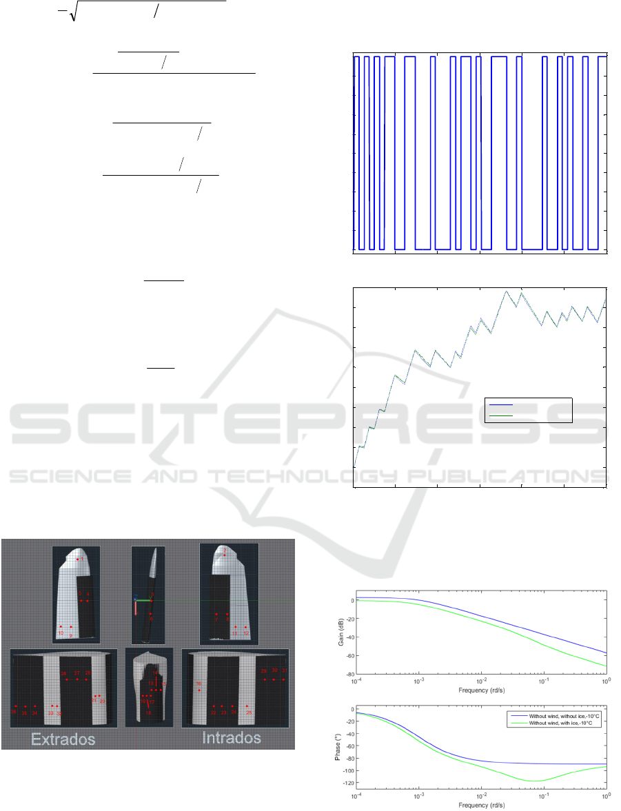
3.2 Parameter Identification

Numerical values of the parameters in relations (1)

and (3) were determined using measures recorded at

31 locations on the prototype as shown on figure 5.

To obtain the measures, a pseudo random binary

sequence (PRBS) shown in figure 6 (top) was used

for the control input u(t).

Figure 5: Locations of temperature sensors (red dots) and

heating paint strips (black) on the prototype.

This dynamic characterization was repeated for

all the thermocouples on the heating strips and for

different wind and ice conditions. As an example,

the frequency responses of the models obtained for

sensor #6 are shown in figures 7 and 8. Similar

results were obtained for the other sensors.

Figure 6: PRBS used for identification and a comparison

of the model response with the measured temperature from

sensor #6 (readjusted at °0C) with ice (T

amb

= – 10°C) and

without wind.

Figure 7: Comparison of the frequency response of the

models obtained for sensor #6, without wind (T

amb

= -

10°C) and with or without ice.

0 500 1000 1500 2000 2500 3000

Time (s )

Control input (V)

0 500 1000 1500 2000 2500 3000

-1

Tim e (s )

Temperature

Model response

Measures

A Solution for Ice Accretion Detection on Wind Turbine Blades

417

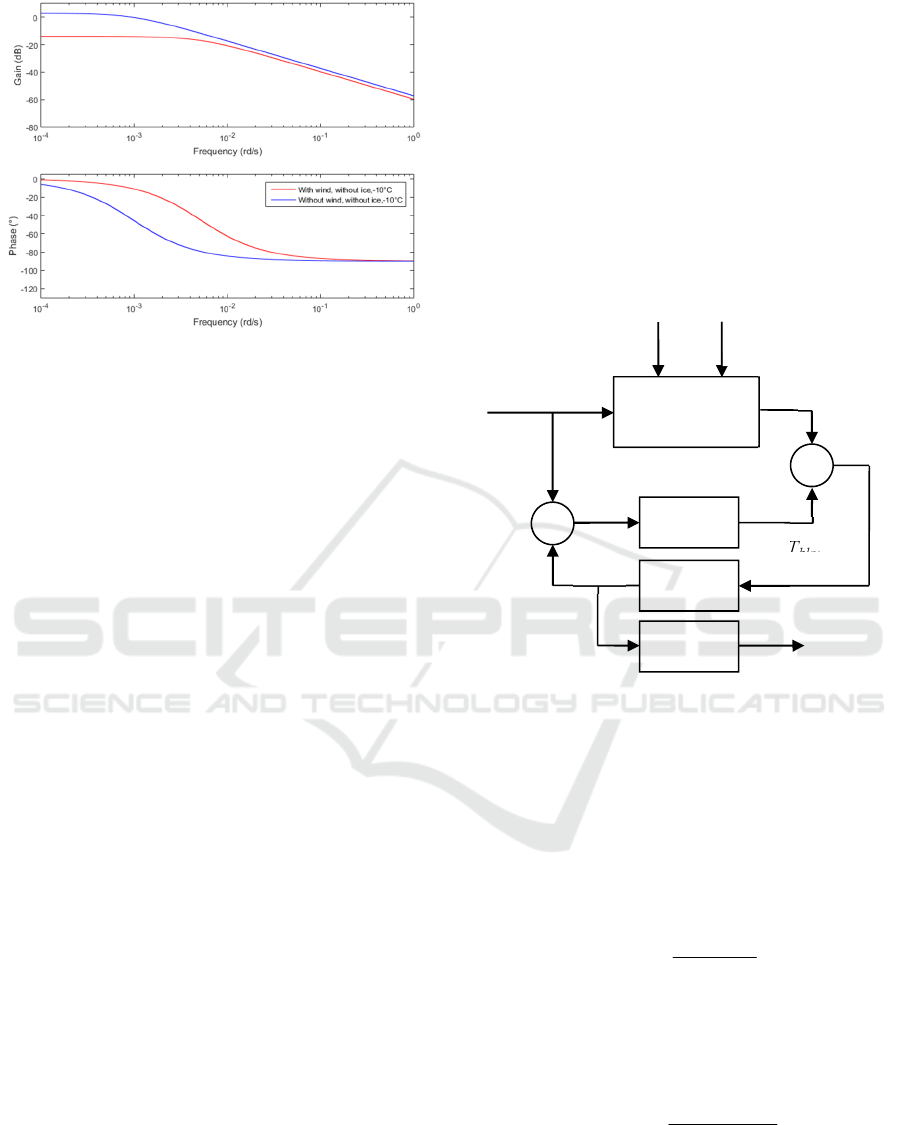
Figure 8: Comparison of the frequency response of the

models obtained for sensor #6, without ice (T

amb

= - 10°C)

and with or without wind (25 m/s speed).

Comparisons of the model frequency responses

reveal that:

- ice on the blade reduces the static gain and the

corner frequency of the frequency responses;

- wind increases the corner frequency of the

frequency responses and in accordance with relation

(1) reduces the static gain through the variation in

the convection exchange coefficient h.

It can be concluded from this comparison that:

- the dynamic behavior variations induced by ice

can be exploited to detect ice accretion,

- wind also creates dynamic behavior variations

that are linked to the convection exchange

coefficient h.

4 ICE DETECTION SOLUTION

The differences in the dynamic behaviors observed

with or without ice and highlighted in the previous

section were next exploited with an observer to

detect ice accretion. The feedback configuration of

the observer means that the control signal, which is

used to deduce ice accretion, can be immunized

against noise and disturbances, while revealing the

significant dynamical behavior differences due to ice

accretion.

4.1 Observer-based Ice Accretion

Detection

The observer-based detection proposed is described

in figure 9. To detect ice, a control input u(t) is

applied to the dimmer that controls the heating of the

paint strips. The resulting signal T

blade

measured by a

temperature sensor is recorded. The same signal u(t)

is applied to the model obtained for the same sensor

without wind and without ice. The estimated

temperature

blade

thus obtained is compared to

blade

to produce an error

. The error is the input of

a controller that modifies the input u(t) to force the

output of the model to cancel the error

. The

higher the output v(t) of the controller, the greater

the difference between the model and the blade ice

accretion state. Signal v(t) after filtering by filter

F(s) can thus be used to decide whether icing occurs

or not.

Figure 9: Observer-based ice accretion detection.

4.2 Validation in a Climatic Chamber:

without Wind

Let G

(s) be the transfer function linking the control

voltage u(t) to the temperature measured by sensor

#6 with

()

0067.0

013.0

. (11)

The numerical values of parameters in relation

(11) are computed to fit time responses in figure 6

through an optimization program. The Z-transform

of G

(s) with a sampling period of 1s is thus

()

9933.01

01296.0

−

zG . (12)

A controller C(z

-1

) was designed to impose a gain

crossover frequency at least 10 times greater than

the corner frequency of G

-1

) on the feedback

Blade with

heating system

and sensors

G(z)

)

C(z)

(z)

Ice accretion

information

blade

∧

v(t)

Wind

speed

amb

ICINCO 2017 - 14th International Conference on Informatics in Control, Automation and Robotics

418

connection of G

-1

) and C(z

-1

). This controller is

given by:

()

3318.03318.11

1574.51045.02619.5

−−

−

+−

−+

. (13)

The following low pass filter

()

99.01

00995.0

−

. (14)

was then tuned (after a Fourier transform analysis)

to attenuate the control input noise. For each test

presented in the sequel, temperature was initially

regulated at -1°C (initial condition) using the system

designed in (Sabatier et al., 2016). A 10V control is

sent to the dimmer to use maximum power to engage

the melting ice very quickly. The time responses

from the sensor (process), the output of the model

(estimated temperature) and at the output of the

controller v(t) in the cases without or with ice are

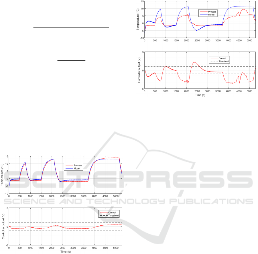
represented respectively in figure 10 and figure 11.

Figure 10: Case without ice: comparison of the

temperature measure from sensor #6 (process) and from

the corresponding model (top) and control signal v(t)

(bottom)

On the ice-free test of figure 10, the blue curve

represents the temperature provided by the identified

model that links the dimmer control voltage to the

temperature measured by sensor #6. This response is

very close to the real temperature that is shown in

red: the error is less than 10% (less than 2 ° C error

for a delta T of 15 ° C). As a result, the control

signal v(t) at the output of the controller remains

below a threshold fixed at 1V.

Figure 11: Case with ice: comparison of the temperature

measure from sensor #6 (process) and from the

corresponding model (top) and control signal v(t)

(bottom).

For the test with ice shown in figure 11, a large

part of the power produced by the paint is absorbed

by the state change in the ice/water and does not

cause an increase in temperature. This leads to a

small static gain for the system linking the dimmer

control voltage and the temperature (thus a

mismatch of the model to the system). Therefore a

negative correction is produced to force the model to

behave like the process. The control signal v(t) at the

output of the controller now exceeds the threshold.

The temperature peaks that occur at times

[≈2000s] and [4500-5000s] correspond to

movements of water and air bubbles in the space

between the ice and the plate. This phenomenon

confirms that the ice is melting. In conclusion, the

detection system of figure 9 produces a control

signal whose level becomes large enough to make it

possible to detect the presence of ice.

4.3 Validation in a Climatic Chamber:

with Wind

With wind, thermal convection needs to be modeled

precisely. The convection coefficient of h (in W. °C

) which appears in figure 4 has to be computed to

parameterize the model in figure 9 as a function of

the wind, and in particular the corner frequency

defined by relation (2). To define the dependence of

on the wind speed (to correctly detect the ice-free

case), a series of characterization tests with a PRBS

dimmer control voltage was carried out for winds up

to 18 m/s. For each test, a model was identified

leading to an estimation of parameter τ = 1/

A Solution for Ice Accretion Detection on Wind Turbine Blades

419

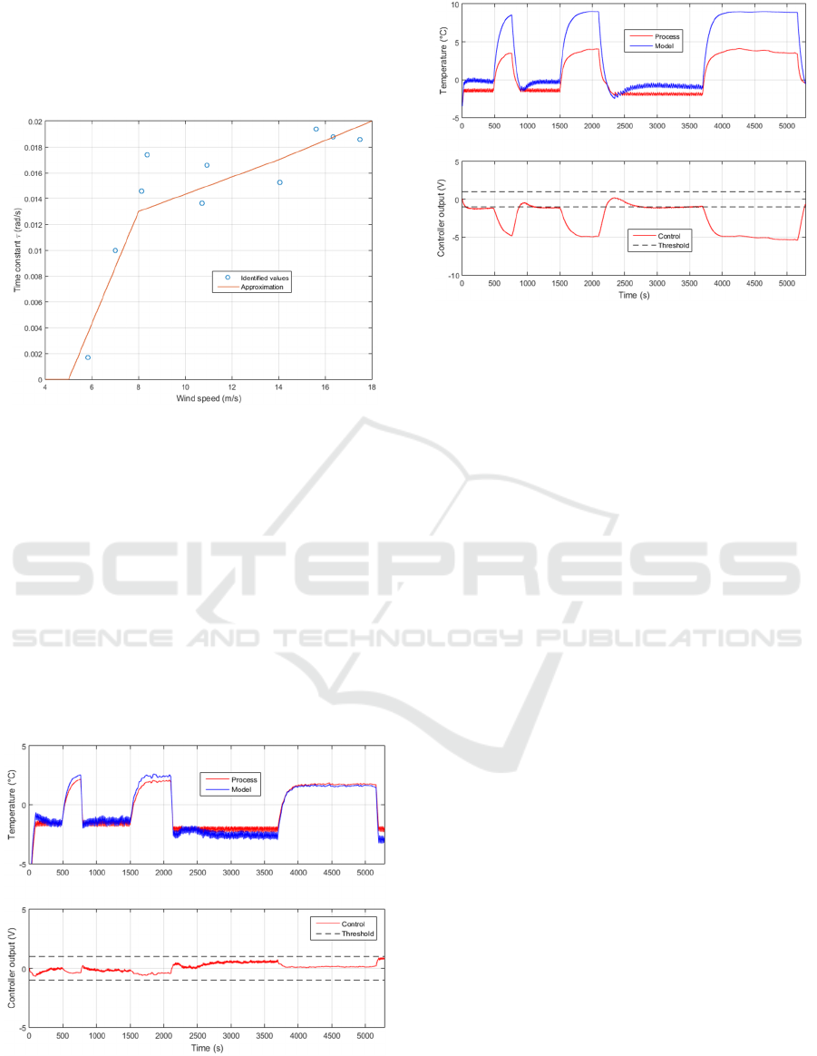
Variations of the time constant

with respect to

wind speed are shown on figure 12 that highlights

the model dependence on the wind speed. This

figure also shows the approximation used in the

model.

Figure 12: Impact of the wind speed on the parameter

= 1/ω

and approximation used in the model.

Given the previous analysis, the corner

frequency of the model G in figure 9 can be adjusted

to take wind conditions (or blade rotation speed) into

account. The results obtained with this strategy are

shown on figure 13 and 14. In figure 13, in spite of

wind conditions and without ice, the control signal

v(t) remains small (less than the 1V threshold) thus

leading to the conclusion of no ice accretion.

Conversely, with ice accretion, figure 14 shows that

the control signal v(t) required to force the model to

behave like the real process is larger than the 1V

threshold. Thus ice accretion can be deduced.

Figure 13: Case without ice and with wind (10 m/s):

comparison of the temperature measure from sensor #6

(process) and from the corresponding model (top) and

control signal v(t).

Figure 14: Case with ice and with wind (10 m/s):

comparison of the temperature measure from sensor #6

(process) and from the corresponding model (top) and

control signal v(t).

These results validate the efficiency of the

proposed method, and especially the relevance of

using an observer to detect the presence of ice. With

ice, the control signal becomes large enough to make

a decision.

5 CONCLUSIONS

Using a de-icing device recently proposed by

(Sabatier et al., 2016) that involves a conductive

polymer paint to heat relevant surfaces of the blade

under electrical potential difference, an ice accretion

detector is proposed. The differences in the

dynamical thermal behavior of the paint with or

without ice accretion are exploited with an observer

to determine whether icing occurs or not. The

proposed strategy was evaluated on a blade

prototype in a climatic chamber. These tests showed

the efficiency of the method both with and without

wind.

REFERENCES

Berbyuk V., Peterson B.; Möller, J., 2014, Towards early

ice detection on wind turbine blades using acoustic

waves, SPIE Proceedings, Vol. 9063.

Botura G., Fisher K., 2003, Development of Ice Protection

System for Wind Turbine Applications, BOREAS VI,

FMI, Pyhätunturi, Finland, p. 16

Dalili N., Edrisy A., Carriveau R., 2009, A review of

surface engineering issues critical to wind turbine

performance, Renewable and Sustainable Energy

Reviews, Vol. 13, pp. 428–438.

ICINCO 2017 - 14th International Conference on Informatics in Control, Automation and Robotics

420

Frohboese P., Anders A., 2007, Effects of Icing on Wind

Turbine Fatigue Loads, Journal of Physics:

Conference Series, Vol. 75.

Ganander, H., Ronsten, G., 2003, Design load aspects due

to ice loading on wind turbine blades. In Proceedings

of the 2003 BOREAS VI Conference. Pyhätunturi,

Finland. Finnish Meteorological Institute.

Hochart, C., Perron J., Fortin G., Ilinca A., 2008, Wind

turbine performance under icing conditions, Wind

Energy, Vol. 11, N° 4, pp 319–333.

Homola M. C., Nicklasson P. J., Sundsbø P. A., 2006, Ice

sensors for wind turbines, Cold Regions Science and

Technology Vol. 46, pp 125–131

Jasinski, W.J., Noe, S.C., Selig, M.S., Bragg, M.B, 1998,

Wind turbine performance under icing conditions.

Transactions of the ASME, Journal of solar energy

engineering, Vol. 120, pp 60–65.

Kimura, S., Sato T., Kosugi K., 2003, The Effect of Anti-

Icing Paint on the Adhesion Force of Ice Accretion on

a Wind Turbine Blade, BOREAS VI, FMI,

Pyhätunturi, Finland, p. 9

Kraj, A. G., Bibeau E. L., 2010, Phases of icing on wind

turbine blades characterized by ice accumulation,

Renewable Energy, Vol. 35, N° 5, pp 966–972

Laakso, T., Peltola E., 2005, Review on blade heating

technology and future prospects, BOREAS VII, FMI,

Saariselkä, Finland, p. 12

Owusu K. P., Kuhn D. C. S., Bibeau E. L., 2013,

Capacitive probe for ice detection and accretion rate

measurement: Proof of concept, Renewable Energy,

Vol. 50, pp 196–205

Parent O., Ilinca A., 2011, Anti-icing and de-icing

techniques for wind turbines: Critical review, Cold

Regions Science and Technology, Vol. 65, N° 1, pp

88–96

Rescoll, 2011, Rescoll Society, web site of the technology

owner, http://www.rescoll.fr/nos_technologies_pani

plast.php.

Ronsten, G., 2004, Svenska erfarenheter av vindkraft i

kallt klimat - nedisning, iskastoch avisning. Elforsk

report 04:13.

Sabatier J., Lanusse P., Feytout B., Gracia S., 2016,

CRONE control based anti-icing / deicing system for

wind turbine blades, Control Engineering Practice,

Vol. 56, pp 200–209

Seifert H., 2003, Technical requirements for rotor blades

operating in cold climate. In Proceedings of the 2003

BOREAS VI Conference. Pyhätunturi, Finland.

Finnish Meteorological Institute.

Skrimpas G. A., Kleani K., Mijatovic N., Sweeney C. W.

Jensen B. B., Holboell J., 2016, Detection of icing on

wind turbine blades by means of vibration and power

curve analysis, Wind Energy, Vol. 19, 1819–1832.

Virk M., Homola M., Nicklasson P., 2010, Effect of Rime

Ice Accretion on Aerodynamic Characteristics of

Wind Turbine Blade Profiles, Wind Engineering, Vol.

34, N° 2, pp 207-218.

A Solution for Ice Accretion Detection on Wind Turbine Blades

421