
Accelerating Square Root Computations over Large GF (2
m
)
Salah Harb and Moath Jarrah
Computer Engineering Department, Jordan University of Science and Technology,
CIT college, P.O.Box 3030, 22110, Irbid, Jordan
Keywords: Cryptosystems, Computation, Elliptic Curve Cryptography, Galois Field, Hardware Implementation, Square
Root.
Abstract: The communication networks of low-resources applications require implementing cryptographic protocols
and operations with less computational and architectural complexities. In this paper, an efficient method for
high speed calculations of square (SQR) root is proposed over Galois Fields GF (2
m
). The method is based on
using the results of certain pre-computations, and transforming the SQR root calculations into a system of
linear equations. The computational complexity of our proposed method for computing the SQR root in GF
(2
m
) is O(m) which is significantly better than existing methods such as Tonelli-Shanks and Cipolla. Our
proposed method was implemented using different types of multipliers over several polynomial degrees.
Software and hardware implementations were developed in NTL-C++ and VHDL, respectively. Our software
experimental results show up to 38 times faster than Doliskani & Schost method. Moreover, our method is
840 times faster than Tonelli-Shanks method. In terms of hardware implementation and since Tonelli-Shanks
requires less resources than Doliskani & Schost, we compare our method with Tonelli-Shanks. The hardware
experimental results show that up to 50% less LUTs with a speedup of 18% that can be obtained compared to
Tonelli-Shanks method.
1 INTRODUCTION
The task of computing square (SQR) roots in Galois
fields GF (p
m
) has a practical importance to the
cryptography such as point counting, the prime-
proving algorithms and asymmetric encryption
scheme in the elliptic curves (ECs) (Menezes, 1993),
where SQR operation is required. In the basic
ELGamal encryption scheme (ElGamal, 1985), a
point P is defined to represent a message on a selected
elliptic curve E
(
x, y
)
over GF (p
m
), where
(
,
)
:y
=x
+ax+b for a,b ∈ GF (p
m
). If M∈
GF (p
m
) denotes the message, then the point P has a
form of (,
(
,0
)
) in a basic cryptographic
scheme.
Finding the points on a curve in EC cryptography
(ECC) requires the SQR root operation. If ∈ GF
(p
m
) is given, the success SQR root =
±
(
++
)
indicates that this point is located
on the curve and applicable for different EC
operations. The SQR root operation is used widely in
compression and restoration points on ECC (Boneh &
Franklin, 2003) (Galbraith, et al., 2003). A point with
coordinates (, ) on the curve is compressed to the
form(, ), where ∈ {0, 1}. To restore the numeric
value () by(, ), it is necessary to solve the
quadratic equation
=
(
)
, which is similar to
compute the SQR root of P
(
x
)
i.e.
()
. As
mentioned earlier, SQR computations of GF (p
m
) is a
significant operation, especially for ECC and other
asymmetric cryptosystems (Galbraith, et al., 2003).
Computing SQR root of the binary GF (2
m
) finite field
is a time-consuming operation. The effectiveness of
cryptosystems that use SQR operations critically
relies on their implementations in finding SQR roots.
With the development of distributed computing in
recent years, the capabilities of computer systems that
can be used in security and critical fields have
significantly increased (Bryen, 2015) (Bitzinger &
Vlavianos, 2016). The simplest measure to improve
security of systems that use GF (2
m
) is to increase the
number of bits (m) in the intermediate operands,
where (m) is the operand length. Usually, the increase
in the number of bits (m) leads to dramatic slowdown
of the performance of cryptographic protection
systems (Barreto & Voloch, 2006). When (m) is
increased, the execution time of SQR operations of
GF (2
m
) is proportionally increased to (
). As a
Harb, S. and Jarrah, M.
Accelerating Square Root Computations Over Large GF (2
m
).
DOI: 10.5220/0006386702290236
In Proceedings of the 14th International Joint Conference on e-Business and Telecommunications (ICETE 2017) - Volume 4: SECRYPT, pages 229-236
ISBN: 978-989-758-259-2
Copyright © 2017 by SCITEPRESS – Science and Technology Publications, Lda. All rights reserved
229

result, the execution time of SQR root operations
increases significantly. Hence, reducing the
execution time of the SQR operation is critical for
practical applications (ElGamal, 1985) (Galbraith, et
al., 2003). In this paper, we propose a new method to
accelerate the SQR root computations using pre-
computed weights over many GF (2
m
) finite fields.
Based on the chosen GF (2
m
), our proposed method
computes the weights only one time and stores them
to be used in data processing. Our experimental
results show high improvements in terms of the
utilized area and the execution time.
2 ANALYSIS OF SQR ROOT
METHODS IN FINITE FIELDS
The practical importance of SQR root computations
in finite fields has resulted in intensive research.
Many methods to compute SQR root that use GF (2
m
)
were proposed with two prominent methods which
are: Cipolla (Cipolla, 1903) and Tonelli (Tonelli,
1891). These methods had been extended to the case
of fields GF (q
m
), where q is a prime, as in Tonelli-
Shanks (Shanks, 1973) and Alderman-Manders-
Miller (L.M. Aldeman & Miller, 1977) methods. In
1977, Tonelli-Shanks method was extended to the
case of extracting the root of arbitrary degrees (L.M.
Aldeman & Miller, 1977) (Z. Cao & Fan, 2011). A
specialized method for computing the cubic root,
characterized by its high speed was developed by (N.
Nishihara & Sueyoshi, 2009).
In Galois fields GF (2
m
), addition and
multiplication are the basic polynomial operations for
the elements {0, (2
m
-1)}. Addition operation
corresponds to a XOR logic and is denoted as '+'.
Multiplication operation in GF (2
m
) consists of two
steps: polynomial multiplication (multiplication
without carry), indicated by the symbol '⊗' and
reduction.
Reduction requires finding the remainder,
denoted as ‘rem’ or ‘mod’, through dividing the
multiplication result by the selected field irreducible
polynomial () of the corresponding degree (m) (I.
Blake & Smart, 1999) (IEEE, 2002). For each
element in GF (2
m
), generated by the irreducible
polynomial
(
)
of degree (m), there is a
multiplicative cyclic group of order (n) that does not
exceed (2
m
-1) (Atkin & F.Morain, 1993) (D.
Hankerson & Vanstone, 2004). The cyclic group of
element i, where (2 ≤ i ≤ 2
m
-1), can be generated by
multiplying the result (s) of a previous element in GF
(2
m
) with i until getting i as a multiplication result
(IEEE, 2002). For example, a GF (2
4
) is formed by
the irreducible polynomial:
() =
+
+1, (P = 25
10
= 110 01
2
),
The cyclic groups are generated in table 1. In each of
the cyclic group of GF (2
m
), a cyclic subgroup can be
found where each element is the SQR of the previous
group. These subgroups of the field that are formed
by a polynomial() =
+
+1 are given
in table 2. Clearly, the order of each of the quadratic
subgroups does not exceed
, which is less than
or equal to (m).
Table 1: Cyclic Groups of the Field GF (2
4
).
Element Cyclic Power Groups
2
2, 4, 8, 9, 11, 15, 7, 14, 5, 10, 13, 3, 6,
12, 1, 2
3 3, 5, 15, 8, 1, 3
4
4, 9, 15, 14, 10, 3, 12, 2, 8, 11, 7, 5,
13, 6, 1, 4
5 5, 8, 3, 15, 1, 5
6
6, 13, 5, 7, 11, 8, 2, 12, 3, 10, 14, 15,
9, 4, 1, 6
7
7, 12, 15, 6, 11, 3, 9, 13, 8, 10, 4, 5, 2,
14, 1, 7
8 8, 15, 5, 3, 1, 8
9
9, 14, 3, 2, 11, 5, 6, 4, 15, 10, 12, 8, 7,
13, 1, 9
10 10, 11, 1, 10
11 11, 10, 1, 11
12
12, 6, 3, 13, 10, 5, 14, 7, 15, 11, 9, 8,
4, 2, 1, 12
13
13, 7, 8, 12, 10, 15, 4, 6, 5, 11, 2, 3,
14, 9, 1, 13
14
14, 2, 5, 4, 10, 8, 13, 9, 3, 11, 6, 15,
12, 7, 1, 14
15 15, 3, 8, 5, 1, 15
Table 2: Quadratic Cyclic Subgroups of the Field GF (2
4
).
Element Power Cyclic Quadratic Subgroups
2 2, 4, 9, 14, 2
3 3, 5, 8, 15, 3
4 4, 9, 14, 2, 4
5 5, 8, 15, 3, 5
6 6, 13, 7, 12, 6
7 7, 12, 6, 13, 7
8 8, 15, 3, 5, 8
9 9, 14, 2, 4, 9
10 10, 11, 10
11 11, 10, 11
12 12, 6, 13, 7, 12
13 13, 7, 12, 6, 13
14 14, 2, 4, 9, 14
15 15, 3, 5, 8, 15
For any GF (2
m
), there is at least one irreducible
polynomial, which implies having different cyclic
SECRYPT 2017 - 14th International Conference on Security and Cryptography
230

groups of two or more irreducible polynomials for the
same GF (2
m
). For example, GF (2
4
) has
another()=
+ + 1, which has cyclic
groups and quadratic subgroups presented in table 3.
In Tonelli-Shanks method, computing
√
A
in GF (2
m
)
requires finding the quadratic cyclic subgroup of A
until the element that is preceding A is found. For
example, according to table 2, if A = 15, the preceding
element in the quadratic sub group is 8, which is the
SQR root of A = 15. Indeed: 88 mod 25 = 64 mod
25 = 15.
Table 3: Cyclic Groups of the Field GF (2
4
).
Element Cyclic Power Groups
Cyclic Quadratic
Subgroups
2
2, 4, 8, 3, 6, 12, 11, 5, 10,
7, 14, 15, 13, 9, 1, 2
2, 4, 3, 5, 2
3
3, 5, 15, 2, 6, 10, 13, 4,
12, 7, 9, 8, 11, 14, 1, 3
3, 5, 2, 4, 3
4
4, 3, 12, 5, 7, 15, 9, 2, 8,
6, 11, 10, 14, 13, 1, 4
4, 3, 5, 2, 4
5
5, 2, 10, 11, 7, 8, 14, 3,
15, 6, 13, 12, 9, 11, 1, 5
5, 2, 4, 3, 5
6 6, 7, 1, 6 6, 7, 6
7 7, 6, 1, 7 7, 6, 7
8 8, 12, 10, 15, 1, 8 8, 12, 15, 10, 8
9
9, 13, 15, 14, 7, 10, 5, 11,
12, 6, 3, 4, 2, 1, 9
9, 13, 14, 11, 9
10 10, 8, 15, 12, 1, 10 10, 8, 12, 15, 10
11
11, 9, 12, 13, 6, 15 -3 14,
8, 7, 4, 10, 2, 5, 1, 11
11, 9, 13, 14, 11
12 12, 15, 8, 10, 1, 12 12, 15, 10, 8, 12
13
13, 14, 10, 11, 6, 8, 2, 9,
15, 7, 5, 12, 3, 4, 1, 13
13, 14, 11, 9, 13
14
14, 11, 8, 9, 7, 12, 4, 13,
10, 6, 2, 15, 5, 3, 1, 14
14, 11, 9, 13, 14
15 15, 10, 12, 8, 1, 15 15, 10, 8, 12, 15
The passage through the quadratic cyclic subgroup is
equivalent to the operation of exponentiation (Z. Cao
& Fan, 2011):
=
()
(1)
Thus, the idea of calculating the SQR root in GF
(2
m
) is theoretically quite simple, but its
implementation involves a significant amount of
computing resources since the calculation of equation
(1) assumes (m-1) operations of root squaring and
reduction. Root squaring follows the rules of
polynomial multiplication, which ignores the carries.
The operation of a polynomial squaring has an
important property: odd-positioned bits of the
squared polynomial of number A are zeros, and the
even-positioned bits are double bits of A, that is, if:
A=
+
.2
+. . +
.2
(2)
T
hen, A
2
is:
AA=
+
.2
+. . +
.2
The importance of this property is that the
calculation of the SQR of a polynomial does not
require any computational overheads, and is basically
a one-position shifting process for the bits in the
initial number. When assessing the computational
complexity of the SQR root operation using Tonelli-
Shanks method, it should be noticed that in practice,
the operand length of the field elements (m)
significantly exceeds the processor word length (l).
Therefore, the elements of the field are divided into t
sections, where t = m / l.
The reduction operation puts the result of a
polynomial multiplication into the limits of the field
GF (2
m
). The polynomial division involves
performing (m-1) cycles. For each cycle, one bit is
shifted in the (m+1)-bit-() code, and added
logically to the current remainder when the last
significant digit is one.
Shifting the (m+1)-bit-() code by one digit
requires (t+1) shift operations. Since this operation is
performed in each of the (m-1) cycles of reduction,
the total number of shift operations is: (t+1).(m-1).
Based on the fact that the reduction operation
involves addition in half of the cycles, the average
number of such operations is (m-1)/2. Implementing
this operation on a l-bit processor requires (t+1)
logical addition operations to be computed.
Therefore, a single reduction operation requires
(t+1).(m-1)/2 operations. Accordingly, the average
running time of a single reduction operation of a SQR
is: 1.5
⋅
(t+1)
⋅
(m-1)
⋅τ
, where (τ) is the execution time
of a single logical operation.
Given that SQR root requires (m-1) squaring
operations, then the average number (N
T
) of logical
operations that are required by the SQR root in GF
(2
m
) is given by equation (3).
=1.5.
(
+1
)
.(−1)
(3)
A similar estimation of the computational
complexity of (
)for Cipolla-Lehmer method is
given in (Menezes, 1993). With the increasing
productivity of distributed computer systems that can
potentially be used in a cryptanalysis system (Feng
Wang & Morikawa, 2005), the easiest way to
improve the reliability of these systems is to increase
the word length of the operands. Increasing operands’
lengths increases the computational complexity
dramatically according to equation (3). Previous
research in calculating the SQR in GF (2
m
) has not
Accelerating Square Root Computations Over Large GF (2
m
)
231
addressed this problem in real implementation of
cryptosystems, which results in higher complexity.
The algorithm that was proposed in (Ozdemir,
2013), has showed improvements in the computation
of the SQR root in finite fields GF (p). The algorithm
is based on a probabilistic theory and gives higher
probabilities of success than the Tonelli-Shanks and
Cipolla algorithms. The algorithm uses polynomial
factorization through locating a random point P over
an elliptic curve
(
,
)
:
=
+; = mP,
where m is an odd integer. If is not the identity point
of the selected curve, then there is a possibility to
obtain the SQR root
√
a
by computing the 2
. value.
The algorithm requires a modular multiplication and
squaring operations for the addition and doubling
calculations. The time complexity in (Ozdemir, 2013)
is
(
)
, where u ≥ 0 is the bit operation for the
EC calculations. The algorithm requires large number
of operations that consume resources and time to
compute the root of a number. The complexity is
increased for large odd values of p.
3 SPEEDING UP
CALCULATIONS OF SQR
ROOT BY STORING MEMORY
WEIGHTS
In practical GF (2
m
) cryptosystems, the generated
polynomials and the used fields are considered fixed.
Keeping this in mind, an effective approach to
accelerate the operation of SQR root in GF (2
m
) is to
use pre-computed weights for the generated
polynomials, where these weights are computed only
one time. The pre-computed weights are stored in
memory and used whenever the SQR root operation
on GF (2
m
) is required. The proposed method is based
on the idea of using the results of pre-computations to
speed up SQR root computations on GF (2
m
). It is
demonstrated as follows:
The number A is represented as a logical sum as:
A = a
+a
.2
+a
.2
+⋯+a
.2
, where
,
,…,
∈ {0,1}. For the logical summation,
the following is valid:
• When n is even, ( + )
=
+
is
true.
• By using equation (1) to calculate the SQR
root of A(B =
√
A
)on GF (2
m
), it can be
re-written as shown in equation (4).
=
(
)
(4)
= (
+
.
(
2
)
+
.
(
2
)
+. . +
.
(
2
)
)
(
)
=
+
.
(
2
)
(
)
+..+
.
(
2
)
(
)
If m values are pre-calculated as:
=1
=
(
2
)
() =
(
2
)
()
=
(
4
)
(
)
=
(
2
)
()
=
(
2
)
(
)
=
(
2
)
()
()
Then the calculation of SQR root in equation (4)
becomes:
=
.
+
.
+⋯+
.
(5)
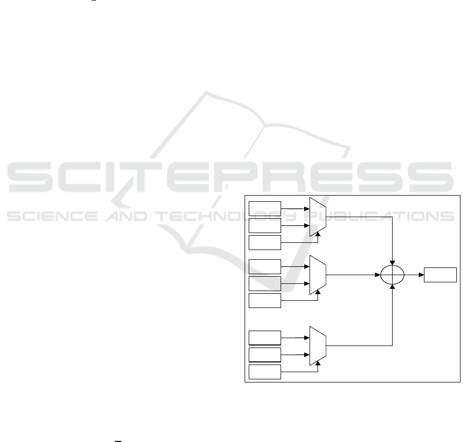
Hence, equation (5) can be directly used to
calculate the SQR root of A. As it is shown in figure
1, once all () weights are generated, each bit ∈
{0, − 1} in A is forwarded to the corresponding
W
. If the x-bit is 1, the weight (
) is selected and
logically added to other selected weights. Otherwise,
the weight is discarded by selecting 0.
0
W
0
a
0
0
1
0
W
1
a
1
0
1
0
W
m-1
a
m
0
1
B
...
Figure 1: Calculation of the square root of input A.
Example: The proposed method is illustrated by the
following example:
Suppose we have GF (2
4
) that is formed using the
polynomial
(
)
=
+
+1, then the pre-
computed weights are:
=1
=
(
2
)
(
+
+1
)
=14
SECRYPT 2017 - 14th International Conference on Security and Cryptography
232
=
(
2
)
(
+
+1
)
=2
=
(
2
)
(
+
+1
)
=5
Assume A = 15 and the bit values of A are:
=
1,
=1,
=1,
=1. To calculate the SQR
root of A, we apply the logical sum operation on the
weights at the one bits of A as:
=
+
+
+
=1+14+2+5=8
Hence, the total number N
of logical operations
that are needed to compute the SQR root using pre-
calculations depends on the number of bits in the
binary code of A. If the number of the one-bits in the
code of A is equal to half of the total number of bits
m, then the value of
is determined by the following
equation (6).
=0.5..
(6)
By comparing expression (6) with expression (3),
we can conclude that the use of the proposed method
to compute the SQR root in GF (2
m
) reduces the
number of operations by a considerable factor which
is almost 1/3m. Consequently, this reduction in the
number of the required operations reduces the
executions time of calculating the SQR root of an
input that uses GF (2
m
).
4 SOFTWARE/HARDWARE
REALIZATIONS AND TIME
EVALUATION
4.1 Software Implementation and Time
Analysis
To prove the correctness and effectiveness of the
proposed SQR root method, a software
implementation for the SQR root method was
developed using C++ programming language with a
special powerful Galois field plug-in called NTL
(NTL, 2016). NTL is a high-performance C++
framework that offers various data structures and
algorithms for manipulating polynomial operations
over integers and finite fields. All computations are
performed using Pentium Dual-Core processor
running on 2.6 GHz clock with 1 GB RAM.
Implementing the proposed SQR root method
involves initially constructing the irreducible
polynomial for GF (2
m
) and creating (m) weights to
calculate the root of A using the logic operation
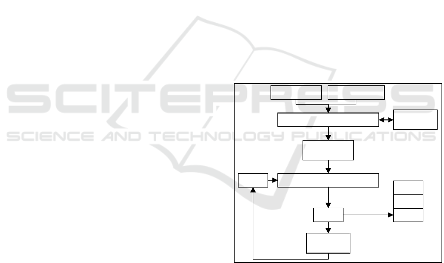
(XOR) or '+'. As shown in figure 2, creating the
weight requires several steps. The first step starts by
taking the constant value 2. Then, the loop (L1)
iterates from 0 to ( − 1) to perform (m) SQR
operations on the constant value 2. This step
computes the base weight (
). The second loop (L2)
iterates from 0 to ( − 2) to perform the
multiplication operation on the base weight (
). At
In each iteration of (L2), the base weight is multiplied
with the previous (
), starting from the base weight
(
).
For example, using a polynomial
(
)
=
+
+1, m=4, we compute:
=1
Using L1 loop:
=14 //
(
2
)
(
+
+1
)
=14
Using L2 loop:
=2 //
(
14
)
(
+
+1
)
=2
=5 //
(
14
)
(
+
+1
)
=5
Once all (m) weights are generated, the third loop
(L3) is executed to calculate the SQR root of A using
a logic operation (XOR). The XOR operation is
executed according to the number of ones in the
binary code of A. This processing step is similar to
applying an on/off process on the weights.
Constant (2) Construct P(x)
Square Operation
L1
(0)
(m-1)
Base Weight
W
1
W
(i-1)
W
(i)
L2
(0)
(m-2)
Multiplication Operation
W
(i)
W
(i-1)
W
(i-2)
Figure 2: Data flow of generating (m) weights.
Table 4 presents an approximate time that is needed
to construct (m) weights using the proposed method
over different GF (2
m
), where (m) is from 16 to 768
bits. The irreducible polynomials for (m) are
generated automatically using a built-in function in
NTL plugin called BuildIrred. As expected, when the
value of (m) increases, the time to generate (m) of
weights increases as well. The execution time to
calculate the SQR root for any m-bit of input A is
Accelerating Square Root Computations Over Large GF (2
m
)
233
almost negligible since the calculations involve only
the logic operation (XOR).
Table 4: Required Time to Generate (M) Weights (NTL).
M Time(sec)
16 0.0017
64 0.0024
128 0.0065
160 0.0073
233 0.0257
512 0.0434
768 0.6391
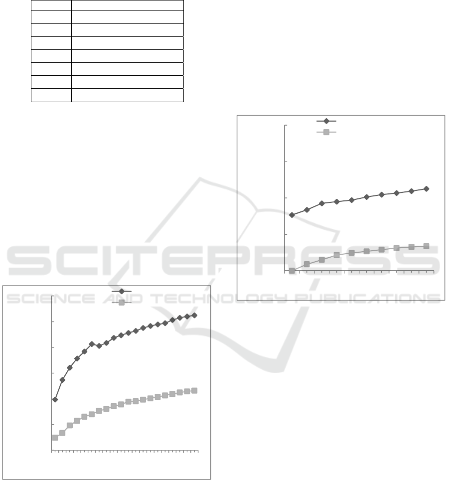
Figure 3 presents an average execution time
comparison between our SQR root NTL
implementation for elements over GF (2
m
), and our
NTL implementation of the famous Tonelli-Shanks
method, where (m) is from 500 to 10000. In each
field, one hundred of random tests were performed for
our method, while ten of random tests were
performed for the Tonelli-Shanks method. As shown
in the figure, our proposed method is much faster than
the Tonelli-Shanks method for all random tests. The
bottleneck of the Tonelli-Shanks method is in the use
of the exponentiation, which takes (m) of squaring
operations to form the cyclic quadratic group for an
element. The method selects the previous element as
the SQR root result.
Figure 3: Average execution time for our proposed method
vs. Tonelli-Shanks algorithm (Software implementation).
On the other hand, our proposed method requires
logic operations (XOR) with one-time pre-
computation of weights. It takes XOR operations
equal to the number of ones at the element or m/2
XOR operations on average.
Figure 4 shows a comparison between our
proposed method over GF (2
m
) and the method of
(Doliskani & Schost, 2014). Both were implemented
in NTL framework. As shown in the figure, our
method outperforms (Doliskani & Schost, 2014)
method in terms of the average execution time. The
average execution time in (Doliskani & Schost, 2014)
is (
(
)
.+
.) when p = 2. This
concludes that our proposed method, which is
O(m/2), does not have bottlenecks in computing the
SQR root for any input over GF (2
m
) due to the logic
operation (XOR). Our method does not need to use
the costly field multiplications, inversions, and
squaring operation.
Figure 4: Average execution time for our proposed method
vs. (Doliskani & Schost, 2014) method (Software
implementation).
4.2 Hardware Implementation,
Resource, and Time Analysis
Basically, our proposed implementation concentrates
on achieving efficient and high-speed SQR root
calculation in Galois fields to improve throughput,
speed, area, and/or power consumption. We have
developed hardware components for the SQR (L1)
and Multiplication (L2) loops that were investigated
in subsection 4.1. These implementations were
developed using VHDL language. The hardware
platform that was used is Xilinx Virtex-5 FPGA
family.
Our implementation is based on equation (7). Two
phases to perform a field multiplication in GF (2
m
)
were applied in order to compute the polynomial
multiplication U(x). A reduction phase is then used on
the selected irreducible polynomial.
Figure 5 shows the average number of LUTs/F.Fs
0,0001
0,001
0,01
0,1
1
10
100
500 2500 4500 6500 8500
Time (sec)
Degree (m)
Tonelli-Shanks
Proposed method
0,0001
0,001
0,01
0,1
1
100 300 500 700 900
Time (sec)
Degree (m)
(Doliskani & Schost, 2014)
Proposed method
SECRYPT 2017 - 14th International Conference on Security and Cryptography
234
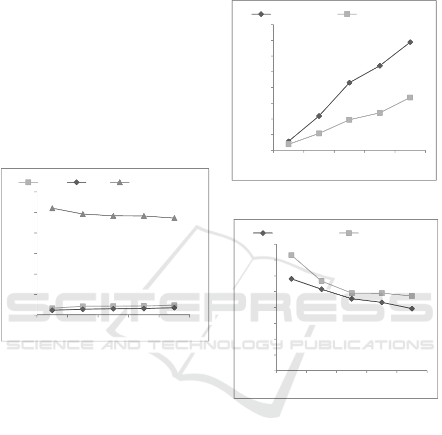
resources and the gained frequencies that are needed
to generate one-time weights for each degree (m)
from 16 to 233 bits. A loop, Karatsuba (Che Wun
Chiou & Lin, 2015) and interleaved multipliers
(Karatsuba & Ofman, 1963) (Rodriguez-Henriquez &
Koc, 2003) (D. Narh Amanor & Schimmler, 2005)
(Gathen & Shokrollahi, 2005) were used to generate
and store weights in order to be used on the received
input data. The process of generating the weights is
performed once. This results in achieving higher
frequencies and less logic elements. Figure 5
illustrates the results.
(
)
=
(
)
(
)
, ℎ
(
)
=
(). ()
(7)
Figure 5: Average number of the required resources using
loop, Karatsuba and interleaved multipliers.
To prove the effectiveness of our SQR root method,
we have implemented it using Xilinx Virtex-5 FPGA
device with values of (m) that range from 16 to 233
bits. Our evaluation involves the efficient Tonelli-
Shanks algorithm since it shows less average
computing time and resources requirements than the
Doliskani & Schost method. Figure 6 and figure 7
compare our method to the Tonelli-Shanks method
over GF (2
m
). As shown in figure 6, our method
requires less LUTs than the Tonelli-Shanks method.
Also, it achieves a higher frequency because of
having only one type of operations (XOR) as shown
in figure 7. The proposed method does not require the
exponentiation operations as in Tonelli-Shanks
method. In Tonelli-Shanks method, the loop
multipliers are used to perform exponentiation
operations. In the
proposed SQR root method, the
weights at a specific selected (m) and an irreducible
polynomial P(x) are generated one time only. In case
of changing the field, a variable can be inserted to
indicate whether to regenerate the weights or not.
Figure 6: Number of LUTs needed in our method vs.
Tonelli-Shanks algorithm.
Figure 7: Achieved frequencies (MHz) in our method vs.
Tonelli-Shanks algorithm.
5 CONCLUSIONS
An efficient and high speed SQR root method over
Galois fields GF (2
m
) is proposed in this paper. It is
based on using pre-calculated weights. The weights
are calculated one time only and then stored in a
storage memory. Software and hardware
implementations were provided in the paper to verify
the proposed method. The computational complexity
of the proposed method is O(m) which is significantly
less than existing methods that require a time
complexity of O(m
2
).
The software implementation of the proposed
method achieves less execution time than both of
520,8
492,4
483,55
483
472,75
0
100
200
300
400
500
600
16 64 128 160 233
Degree (m)
LUTs F.Fs Frequency (MHz)
58
219
431
539
689
39
108
195
239
337
0
100
200
300
400
500
600
700
800
16 64 128 160 233
Number of LUTs
Degree (m)
Tonelli-Shanks Proposed method
290,639
257,839
227,844
216,38
196,647
365,43
283,476
245,621
245,317
236,583
0
50
100
150
200
250
300
350
400
16 64 128 160 233
Frequency (MHz)
Degree (m)
Tonelli-Shanks Proposed method
Accelerating Square Root Computations Over Large GF (2
m
)
235

Tonelli-Shanks and Doliskani & Schost methods
using several random tests. The hardware
implementation uses different types of multipliers
including loop, Karatsuba, and interleaved
multipliers. The experimental results show that our
method outperforms the Tonelli-Shanks method over
GF (2
m
) in terms of the required resources and
frequencies using several polynomial degrees.
ACKNOWLEDGEMENTS
This work is supported by the Deanship of Research
at Jordan University of Science and Technology grant
number 20160227/89-2016.
REFERENCES
Atkin, A. & F.Morain, 1993. Elliptic curves and primality
proving. Math. Comput, 61(203), pp. 29-68.
Barreto, P. S. L. M. & Voloch, J. F., 2006. Efficient
Computation of Root in Finite Fields. Designs, Codes
and Cryptography, 39(2), pp. 275-280.
Bitzinger, R. & Vlavianos, H., 2016. Emerging Critical
Technologies and Security in the Asia-Pacific. 1st ed.
s.l.:Palgrave Macmillan.
Boneh, D. & Franklin, M., 2003. Identity-Based Encryption
from the Weil Pairing. SIAM J. of Computing, 32(3),
pp. 586-615.
Bryen, S. D., 2015. Technology Security and National
Power: Winners and Losers. 1st ed. s.l.:Transaction
Publishers.
Che Wun Chiou, C.-Y. L. J.-M. L. Y.-C. Y. H. W. C. & Lin,
L.-C., 2015. Digit-Serial Systolic Karatsuba Multiplier
for Special Classes over GF(2m). Journal of
Computers, 26(1), pp. 40-57.
Cipolla, M., 1903. Un metodo per la risolutione della
congruenza di secondo grado. Rendiconto
dell’Accademia Scienze Fisiche e Matematiche, 9(3),
pp. 154-163.
D. Hankerson, A. M. & Vanstone, S., 2004. Guide to
elliptic curve cryptography. In: New York: Springer-
Verlag.
D. Narh Amanor, C. P. J. P. V. B. & Schimmler, M., 2005.
Efficient hardware architectures for modular
multiplication on FPGAs. s.l., International Conference
on Field Programmable Logic and Applications, pp.
539-542.
Doliskani, J. & Schost, É., 2014. Taking roots over high
extensions of finite fields. Mathematics of
Computation, Volume 83, pp. 435-446.
ElGamal, T., 1985. A public key cryptosystem and a
signature scheme based on discrete logarithms. IEEE
Trans. Inform. Theory 31, Issue 4, pp. 469-472.
Feng Wang, Y. N. & Morikawa, Y., 2005. A high – speed
square root computation in finite fields with application
to elliptic curve cryptography. Mem Fac Eng Okayama
Univ, Volume 39, pp. 82-92.
Galbraith, S., Paulus, S. & Smart, T., 2003. Arithmetic on
superelliptic curves. Mathematics of Computation,
32(237), pp. 393-405.
Gathen, J. v. z. & Shokrollahi, J., 2005. Efficient FPGA-
based Karatsuba multipliers for polynomials over F2.
s.l., Proc. 12th Workshop on Selected Areas in
Cryptography (SAC 2005),, pp. 359-369.
I. Blake, G. S. & Smart, N., 1999. Elliptic curves in
cryptography, Cambridge: Cambridge University
Press.
IEEE, 2002. Standard specifications for public-key
cryptography. [Online]
Available at: http://grouper.ieee.org/groups/1363/
[Accessed July 2016].
Karatsuba, A. & Ofman, Y., 1963. Multiplication of
Multidigit Numbers on Automata. Soviet Physics-
Doklady, 7(7), pp. 595-596.
L.M. Aldeman, K. M. & Miller, G., 1977.
On taking root in
finite fields. Providence, RI, Proc. 18-th IEEE
Symposium on Foundations of Computer Science.
Lehmer, D., 1969. Computer technology applied to the
theory of numbers. Number Theory, Math. Assoc.
Amer, p. 117–151.
Menezes, A. J., 1993. Elliptic Curve Public Key
Cryptosystems. Volume 234, pp. 14-128.
N. Nishihara, R. H. & Sueyoshi, Y., 2009. А remark on the
computation of cube root in finite fields. [Online]
Available at: http://eprint.iacr.org/2009/457.pdf
[Accessed June 2016].
NTL, 2016. NTL: A Library for doing Number Theory.
[Online]
Available at: http://www.shoup.net/ntl/
[Accessed July].
Ozdemir, E., 2013. Computing Square Roots in Finite
Fields. TRANSACTIONS ON INFORMATION
THEORY, 59(9), pp. 5613-5615.
Rodriguez-Henriquez, F. & Koc, K., 2003. On Fully
Parallel Karatsuba Multipliers for GF(2m). s.l., Proc.
Int’l Conf. Computer Science and Technology (CST
2003), p. 405–410.
Shanks, D., 1973. Five number-theoretic algorithms.
Winnipeg, Man, Congressus Numerantium.
Tonelli, A., 1891. Bemerkung über die Auflösung
quadratischer Congruenzen. Göttinger Nachrichten, pp.
344-346.
Z. Cao, Q. S. & Fan, X., 2011. Adleman-Manders-Miller
root extraction. [Online] Available at:
http://arxiv.org/abs/1111.4877 [Accessed June 2016].
SECRYPT 2017 - 14th International Conference on Security and Cryptography
236
