Land Change Modeling Handling with Various Training Dates

Martin Paegelow

Department of Geography, Université de Toulouse Jean Jaurès, 5 allées A. Machado, 31058 Toulouse, France

Keywords: Land Change Modeling, Training Dates, Validation.

Abstract: Popular modeling tools for land change simulation, especially those using Markov chains, undertake model

training based only on two land use / cover (LUC) maps. This paper analyses uncertainty and potential

errors caused by taking into account only two former, model known, LUC maps. This is illustrated by a

simple data set of six LUC maps allowing various Markovian transition matrices; a range even larger by

considering different confidence levels. Results underline the randomness in choice of only two training

dates. Authors propose alternative methods to Markov chains integrating all available LUC maps in order to

simulate forecasting scenarios. To do so, they incorporate all possible LUCC (land use / cover change)

budgets to perform simple arithmetic combinations between the six training dates. Comparing Markov chain

transitions based on two training dates and alternatively performed change rates taking into account all

training dates results to important differences. This study underlines the importance of the choice of training

dates during model calibration for path-dependent simulations.

1 INTRODUCTION

Land change modeling consists in simulation of its

change in terms of quantity and allocation. The

amount of changes during the simulation step

depends on the modeling objective. For plausible

land change scenarios, the modeler designs different

solutions implementing alternative hypotheses about

future (e.g. business as usual scenario, sustainable

development scenario, …) and therefore introduce

various quantities of LUC. In this context, the model

answers the question ‘what will be the spatial

impact if so?’. At the opposite, if the objective is

prediction or forecasting, expected LUC or transition

quantities are calculated. Quantity prediction is often

done by probabilistic approaches such as Markov

chains. Some geomatic LUCC modeling software

such as CA-Markov, Land Change Modeler (both

implemented in Terrset) and Dinamica Ego (Mas et

al., 2014) but also LucSim calculate Markovian

conditional transitions. They perform this

extrapolation in time by using only two training

dates (TD). This is a risk-taking approach because

model training depends on only two time points in

the past. What happens if at least one of the two TD

does not match key points in the time series.?

Considering only two maps as a long time series also

increases the impact of data error due to

classification or photo interpretation. Several studies

emphasize the impact of temporal data resolution

(Allen and Starr, 1982, Kim, 2013) and study the

impact of time intervals on the amount of change

(Burnicki et al., 2007, Lee et al., 2009, Lieu & Deng,

2010). The authors note that n-order Markov chains

are currently employed, often in a spatially non

explicit context. Generally, these n-order MC are

based on a rather eventful multi-temporal database

(cf. Ju et al., 2003). Nevertheless, n-order MC are

more complex to handle and not included in popular

GIS software.

Authors present test areas and data before

illustrating the random character by taking into

account only two training maps. Then they test

simple techniques to introduce multitemporal

knowledge in predictive models. Authors do this at

global and categorical as well as on transition level.

Coupling different training dates (TD) and

confidence levels within a Markov chain process as

proposed alternatives integrating more than two TD

may inform the modeler when designing simulation

models.

2 TEST AREA AND DATASET

The test area is an 8 750 ha catchment located in the

western part of the French Department Pyrénées

Orientales called Garrotxes. The altitude ranges

350

Paegelow, M.

Land Change Modeling Handling with Various Training Dates.

DOI: 10.5220/0006385003500356

In Proceedings of the 3rd International Conference on Geographical Information Systems Theory, Applications and Management (GISTAM 2017), pages 350-356

ISBN: 978-989-758-252-3

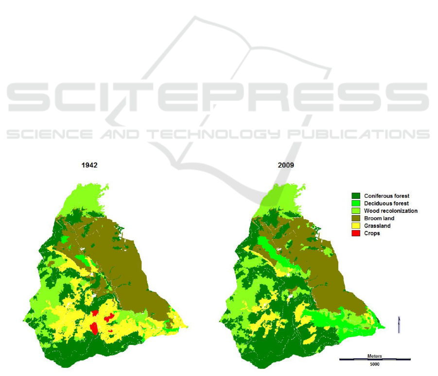
from 650m (SE, Mediterranean climate) to 2400 m

(N, mountain climate). The western part, on granitic

substratum, was used for agriculture and is mostly

wooded today while the eastern bank, overlying

schist, forms large summer pastures. The population

of the 5 municipalities pulled down from 1 832

habitants in 1826 to about 100 today. At the

beginning of the 19

century about a quarter of land

was used by crops on terraces (Napoleon cadaster).

Afterwards crops, currently marginal, became

transformed into pasture, shrubs or woody land.

Actual activities are pasture, timber extraction and

touristic activities.

The data set employed consists in six LUC maps

of years 1942, 1962, 1980, 1989, 2000 and 2009.

These LUC maps result from image segmentation

and supervised classification on ortho-photographs

with visual post validation.

3 METHODOLOGY

3.1 Measuring the Impact of Multiple

Training Dates (TD)

Land change is analysed by the technique of LUCC

budget (Pontius et al., 2004b and 2008). Its

components gain, loss, total change, net change and

swap are calculated for the five periods of the

training LUC maps time series. Authors convert

coarse time interval dependent indicators into mean

annual rates for comparison.

Most quantity prediction in business as usual

(BAU) simulation scenarios are performed by using

Markov (first order Markov chain) where t1 and t2

are TD and T the simulation date. To highlight the

impact of TD, authors test both: various

combinations of two TD for MC transition matrices

and different confidence in these training data. First

we form all possible pairs of TD possible pairs of

TD except the last one (2009). For each of these

pairs we compute MC expected transitions for model

unknown T (2009). We refine this analysis by

introducing two confidence levels applied to input

training data. The default option of several software,

consisting in applying 0.0 % of proportional error is

compared to 90% confidence level (proportional

error of 0.1).

In parallel, authors compute the overall and LUC

specific annual change rates (%).

3.2 Computing Transition Rates

including All TD versus Markov

Chains

Authors propose some alternative and simple

techniques to extrapolate future LUC by computing

transition matrices between 2009 (last known date)

and 2020 (simulated LUC) using all known LUC

maps. This means that our approach includes five

training periods (six TD). These techniques only

differ by weighting the impact of individual training

periods. The starting point are observed annual

transition rates by period.

Figure 1: Garrotxes test area. LUC in 1942 and 2009.

Land Change Modeling Handling with Various Training Dates

351

Weighing of multiple transition periods:

 Average: the sum of transition rates over

six TD for a specific cell into the transition

matrix for T is divided by the number

considered periods (five).

 Time distance weighted average: the impact

of a period decreases proportionally with

remoteness to the present. For a series of n

time intervals, the weight of the farthermost

time interval equals 1, the weight of the

most current time interval equals n. The

annual rates are this way weighted and

summed before being divided by the sum of

weights. Authors are conscious that this

weighting scale could be enhanced by

numerous ways such as considering equal

time intervals or varying individual weights

by the corresponding length of interval.

where sum of weights:

 Linear trend: the best linear fit (linear

regression)

 Exponential trend: weights are obtained by

geometric exponential trend

Every weighting technique is applied to each

transition except persistence (diagonal cells). To

compute cross-tabulation for expected changes,

authors:

o Define a simulation date: 2020. This means

last known LUC (2009) updated by 11

times expected annual change rate. Because

crops disappeared completely during the

1980ties, the corresponding column and

row in the transition matrix for 2020 is set

to zero by reporting proportionally missing

pixels on the rest of the table.

o At this state extrapolated persistence

(diagonal cells) is missing in the transition

matrix. Authors fill each diagonal cell by

the number of cells of concerned LUC in

2009 (starting date of simulation) minus the

sum of transitions from this category to

other categories.

The last step is comparing these all TD englobing

transition matrices to classic MC transitions

based only on two TD. Among the many

possibilities, authors chose two couples of

TD for MC based transition matrices: the

pair formed by most recent dates (i.e. 2000

– 2009 to simulate expected changes for

2020) and the pair forming the recent

period closest to the average of all periods

(i.e. 1989 – 2009).

4 RESULTS

4.1 Measuring the Impact of Multiple

Training Dates (TD)

4.1.1 LUCC Budgets

For each of the five training periods LUCC budgets

were computed. Because periods have different

lengths, results are expressed as annual rates. For

total change, the mean annual rate was less than 20

ha / year during the 1980s while exceeding 40 ha /

year through the periods 1962 – 1980 and 1989 –

2000. The fraction of net change is differing from

less than 50 % (1980s) up to 90 % during the last

period. During the three other periods net change

was about 75 % of total change. LUCC budgets

show that land change and particularly the

proportion of net change to swap was not linear

during the last seven decades.

When considering change rates on the

categorical level, the situation is even more

contrasting. First most dynamic periods (1962 –

1980; 1989 – 2000) on the global level are only the

most dynamic for coniferous forest. Other LUC

categories show different trends: evidently broom

land becomes more dynamic with time while

decreasing for grassland. Deciduous forest had two

more dynamic periods (1942 – 1962 and 1989 –

2000) whereas results for crops are difficult to

interpret of cause disappearing during the period

1980 – 1989. We also notice different levels of

change rates depending on LUC categories. Wood

recolonization is the most dynamic category while

coniferous and deciduous forest are more stable.

4.1.2 Markov Chains and Variation of

Confidence Levels

When considering the penultimate date (2000) as

last training date in order to extrapolate on the last,

model unknown, date (2009) to allow comparisons

with real LUC in 2009, ten MC couples may be

constituted. For instance, beginning with 1942, we

GAMOLCS 2017 - International Workshop on Geomatic Approaches for Modelling Land Change Scenarios

352

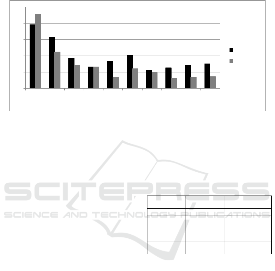
Figure 2: Absolute differences between 2009 observed and 2009 Markov chain (proportional error 0.0 and 0.1) predicted.

have four possibilities (selecting 1962, 1980, 1989

or 2000 as second training date) to perform Markov

chain while the date of 1989 as starting point only

offers 2000 as second training date.

All ten Markov chains were computed twice:

first with a 0.0 % proportional error, then with 10 %

proportional error in order to analyze the impact of

confidence in data. We compared Markov chain

predicted LUC with 2009 observed LUC and we

added the absolute difference predicted minus

observed for each category shown in fig. 2.

Considering the 100 % confidence level in LUC

maps, the choice of a couple of TD makes that the

quantitative prediction error may be near to 5 %

(choosing 1980 and 200) or almost four times higher

(1942 and 1962). We notice that limited confidence

in training data (10 % error) give in nine MC out of

ten closer results to observed LUC in 2009 as entire

confidence in data.

4.2 Computing Transition Rates

including All TD versus Markov

Chains

The comparison of the four alternative simulated

transition rates for 2020 (average, time distance

weighted average, linear and exponential trend) and

two Markov chain matrices (one considering 1989

and 2009 as TD, the other 2000 and 2009, cf.

methodological section) of expected changes to

2020 shows that global persistence is very uniform

and important (varying from 95.06 to 96.71 %). At

the categorical level, the comparison leads to more

contrasted results as summarized in table 1.

Table 1: Absolute differences (% of entire area) between

Markov chain (MC) performed transition matrices and

four alternative methods (alternatively computed by

average, time distance weighting, linear or exponential

trend) including the entire set of available TD for 2020.

For each comparison, we summed the absolute differences

of transition rates between the different LUC categories.

The left column shows the difference based on MC using

1989 and 2009 as TD while the right column indicates

differences based on MC using 2000 and 2009 as TD.

(1989-2009)

(2000-2009)

Average

2.04

6.24

Time dist-

ance weighted

0.95

5.02

Linear

trend

5.37

9.88

Exponenti

al trend

3.36

7.36

Table 1 inform us that the differences are less

important while using Markov chain transitions for

2020 based on a training period close to the average

of total time extent (1989 – 2009, left) than

considering the last available training period (2000 –

2009, right). For each pair of TD, Markov chain

predicted transitions are closest to time distance

weighted average as technique integrating all TD.

The most important differences result from

comparison Markov minus Linear Trend.

Fig. 3 informs us about differences on the

transitional level. Here we examine differences for

individual transitions between alternative method

and MC based last available TD (2000 and 2009).

Graphics in fig. 3 show the difference between

Markov chain expected transition rates (%) and

alternatively performed transition rates (%). A

1942 -

1962

1962 -

1980

1980 -

1989

1989 -

2000

1942 -

1980

1962 -

1989

1980 -

2000

1942 -

1989

1962 -

2000

1942 -

2000

0 % error

10% error

Land Change Modeling Handling with Various Training Dates

353

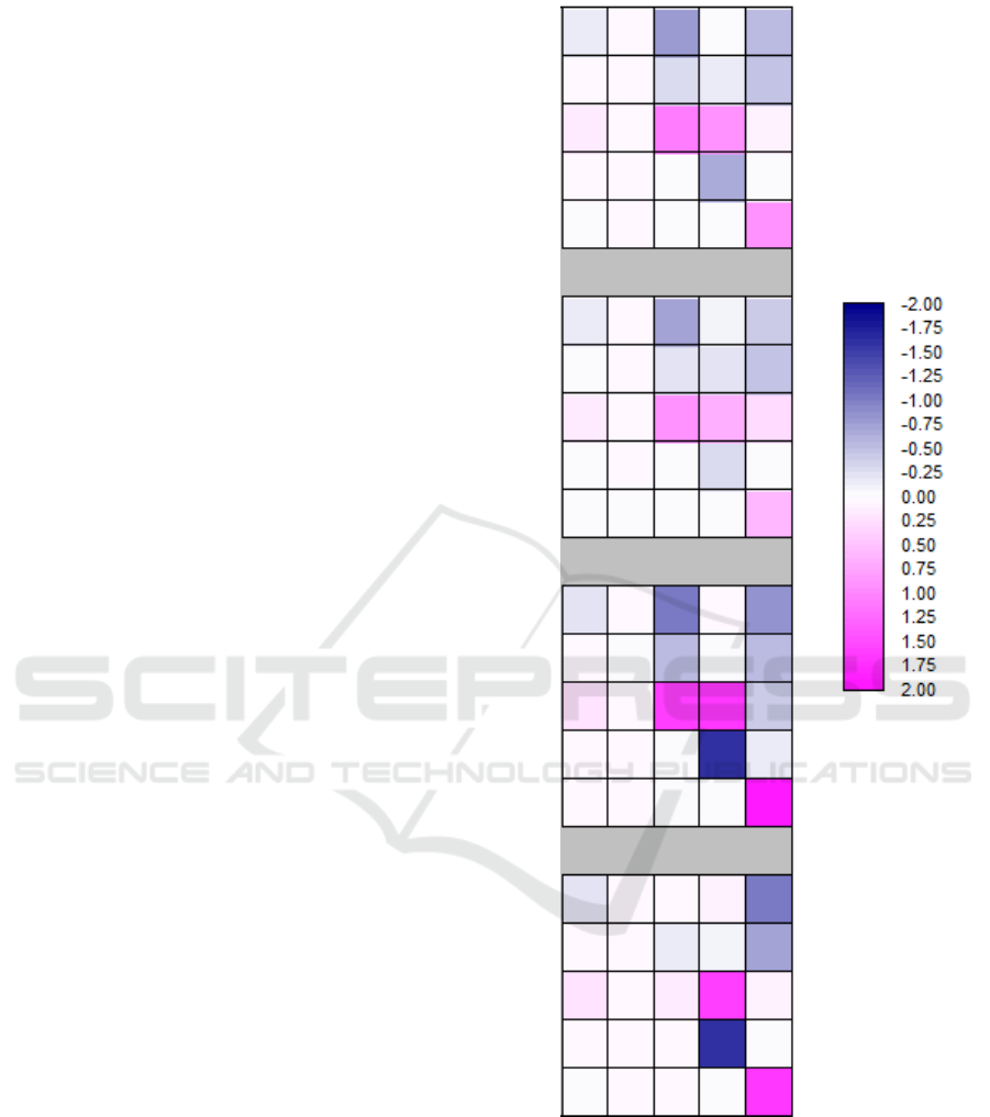
positive number means that Markov chain simulated

transition is more voluminous. A negative result

indicates that Markov chain predicted transition

affects less surface than alternatively calculated. At

the individual transition level, fig. 3 points out that:

 Differences do not surpass more than 2 %

of total area.

 Differences affects in a specific way LUC

transitions: especially wood recolonization

(third row) is a ‘gaining category’. This

means that Markov chain predicted amount

of change is higher than alternatively

calculated amount of change. On the other

hand, transitions from grassland to other

LUC (fifth column) are generally negative

(i.e. alternatively computed transition rates

are more voluminous than by Markov

chain) while persistence (lowest right cell)

balances this.

5 DISCUSSION

Various approaches intend to analyze occurred land

change in order to simulate those in the future.

Authors quote the wide field of techniques able to

describe dynamics such as LUCC – budget (Pontius,

2000; Pontius et al., 2004a, 2004b) and intensity

analysis (Aldwaik & Pontius, 2012; Pontius et al.,

2013). Other techniques such as sensitivity analysis

(Pontius et al., 2006; Jokar Arsanjani et al., 2012,

Paegelow et al., 2014) target to test the robustness of

model data and drivers by analyzing, among other

aspects, the significance of used data such as TD.

5.1 Measuring the Impact of Multiple

Training Dates (TD)

LUCC budgets underline that land change was not a

linear process and its composition either. In this

context, it is important to notice that computed

LUCC budget indicators are quite average land

change indicators. As mentioned, the situation is

even more contrasted on the categorical level as

illustrated for the mean annual net gain (ha) of

coniferous forest expressed in fig. 4. If the modeler

chooses 2000 and 2009 as TD for a BAU scenario,

the amount of simulated land change will be less and

specific net gain for coniferous forest near zero.

However, during this period (2000 to 2009) land

changed tending towards forest. The average net

gain for wood recolonization was the highest one for

this period. At the opposite, if the modeler takes

1962 and 1980 as TD, the BAU scenario would be

Figure 3: Differences between Markov chain (TD: 2000

and 2009) predicted and alternatively calculated transition

rates for 2020. Each square presents one comparison. Top

matrix compares MC to average, second to time distance

weighted, third to linear trend and fourth (bottom) to

exponential trend. Each matrix compares individual

transitions. Because crops are absent, each cross tabulation

matrix is composed by only five columns and rows. From

left to right / top to down: coniferous forest (1), deciduous

forest (2), wood recolonization (3), broom land (4) and

grassland (5), cf. numbers on the top matrix.

GAMOLCS 2017 - International Workshop on Geomatic Approaches for Modelling Land Change Scenarios

354

very dynamic while wood recolonization was

registering an average net loss of about 9.6 ha / year.

This example shows both, that the most actual

data are not even representative and that land change

for a specific land use / cover category cannot be

understood if disconnected from other.

Transitions simulated by Markov chains (MC)

and comparison to observed land change points out

that the most recent TD are not per se the closest to

reality. At the opposite, this data set underlines that

the use of the last available training date (2000)

reduces the absolute difference between observed

and MC predicted LUC and this independently of

the duration of the training period.

Figure 4: average annual net gain in ha of coniferous

forest per period.

Knowing that the choice of TD for MC

prediction determines quantitative accuracy of BAU

scenarios, disposing of only two TD may lead to

random results still increased by applying different

confidence levels to training data.

The comparison by period of average annual

transition rates at global level and categorical level

(Fig. 2) illustrate the heterogeneity of speed and

tendencies in land change. The choice of accurate

TD is complex and picking only two TD may

exceedingly impoverish real dynamics. To

overcome this problem, authors propose alternative

forms consisting in the integration of multi temporal

data as training basis of quantitative simulation.

5.2 Computing Transition Rates

including All TD versus Markov

Chains

The integration of multiple TD exhibits the

possibility to overcome the two TD restriction of

commonly used MC to quantitative land change

prediction. Results on this data set are, depending on

weighting individual dates, rather close to MC

generated transition matrices. This effort to compare

them underlines the methodological difficulty to

relate a 2 TD based approach to another one

integrating 2 + n TD. The Markovian choice of a

couple of dates unavoidably induces data reduction.

On the other hand, taking into account a memory in

the simulation process by proposed alternatives is,

theoretically, an improvement. In contrast, using all

available LUC maps necessitate to supervise this

process to avoid illogical transitions as shown for

crops for this data set and may make adjustments

necessary.

Applied weighting techniques are still a small

and simple sample among a wide range of

possibilities. Because of necessary supervision, we

consider that applying these alternative techniques

are nearby to the frontier between land change

prediction and forecasting scenarios.

6 CONCLUSION

In simple words, land change models accomplish

only two tasks: calculating expected quantities and

allocating them into the map. With regard to the first

task a considerable number of studies reveal the use

of Markov chain simulated transitions based only on

two training dates. This contribution first highlights

the randomness of picking out two training dates

when disposing of a larger series or the uncertainty

when holding only two dates and its consequences

on Markov chain predicted land change. The

complexity of LUCC is illustrated by computing

annual transition rates on three levels: global,

categorical and transitional. Subsequent, authors

describe simple alternative methods to overcome

Markov chains, considering only one training

period, by using all available dates and weighing

them differently. This approach generates a new

difficulty. Modelers have to supervise and, if

necessary, adjust the generation of transition

matrices to avoid illogical transitions. The range of

results underlines the caution that must show a

modeler and the critical sense with which recipients

have to interpret correctly a simulation that is never

more than a plausible future. Therefore, one key for

correct understanding is transparency on both:

available as used data for potential and operated

methodological choices.

Land Change Modeling Handling with Various Training Dates

355

ACKNOWLEDGEMENTS

This work was supported by the BIA2013-43462-P

project funded by the Spanish Ministry of Economy

and Competitiveness and by the Regional European

Fund FED.

REFERENCES

Aldwaik S.Z. & Pontius Jr. R.G., 2012, Intensity analysis

to unify measurements of size and stationaity of land

changes by interval, category, and transition,

Landscape and Urban Planning 106, 103-114

Allen T.H.F. and Starr B., 1982, Hierarchy: Perspectives

for ecological complexity. University of Chicago

Press. Chicago, 310 p.

Burnicki A.C., Brown D.G. and Goovaerts P., 2007,

Simulating error propagation in land-cover change

analysis: The implications of temporal dependence.

Computers, Environment and Urban Systems 31, 282–

302

Camacho Olmedo M.T., Pontius Jr. R.G., Paegelow M.,

Mas J.F , 2015, Comparison of simulation models in

terms of quantity and allocation of land change.

Environmental Modelling & Software, v. 69 May

2015, p. 214-221.

Gómez Delgado, M. and Tarantola, S., 2006, “Global

sensitivity analysis, GIS and multi-criteria evaluation

for a sustainable planning of hazardous waste disposal

site in Spain”. International Journal of Geographical

Information Science, 20, 449-466.

Hu G., Hu J., Zhang C., Zhuang L., Song J., 2003, Short-

term traffic flow forecasting based on Markov chain

model. In: Intelligent Vehicles Symposium 9-11 June

2003. Proceedings IEEE, pp. 208-212.

Jokar Arsanjani, J., 2012, Dynamic Land-Use/Cover

Change Simulation: Geosimulation and Multi Agent-

Based Modelling, Springer Theses, Springer Verlag.

Kim J.H., 2013, Spatiotemporal scale dependency and

other sensitivities in dynamic land-use change

simulations. International Journal of Geographical

Information Science 27, 1782–1803

Lee Y.J., Lee J.W., Chai D.J., Hwang B.H. and Ryu K.H.,

2009, Mining temporal interval relational rules from

temporal data. Journal of Systems and Software 82,

155–167

Liu J. and Deng X., 2010, Progress of the research

methodologies on the temporal and spatial process of

LUCC. Chin. Sci. Bull. 55, 1354–1362

Mas J.F., Kolb M., Paegelow M., Camacho Olmedo M.T.,

Houet T., 2014, “Inductive pattern-based land

use/cover change models: A comparison of four

software packages”. Environmental Modelling &

Software, v 51 January 2014 P.94-111

Paegelow M., Camacho Olmedo M.T., Mas J.F., Houet T.,

2014, Benchmarking of LUCC modelling tools by

various validation techniques and error analysis.

Cybergeo, document 701, mis en ligne le 22 décembre

2014. URL : http://cybergeo.revues.org

Pontius Jr. R.G., 2000, “Quantification error versus

location error in comparison of categorical maps”.

Photogrammetric Engineering & Remote Sensing, 66

(8), 1011-1016.

Pontius Jr. R.G., Huffaker, D., Denman, K., 2004a,

„Useful techniques of validation for spatially explicit

land-change models”. Ecological Modelling, 179 (4),

445-461.

Pontius Jr. R.G., Shusas E. and McEachern M., 2004b.

Detecting important categorical land changes while

accounting for persistence. Agriculture, Ecosystems &

Environment 101(2-3) p.251-268

Pontius Jr R.G., Boersma, W., Castella, J.C., Clarke, K.,

de Nijs, T., Dietzel, C., Duan, Z., Fotsing, E.,

Goldstein, N., Kok, K., Koomen, E., Lippitt, C.D.,

McConnell, W,, Sood, A.M., Pijankowski, B.,

Pidhadia, S., Sweeney, S., Trung, T.N., Veldkamp,

A.T., Verburg, P.H., 2008, “Comparing the input,

output, and validation maps for several models of land

change”. Annals of Regional Science, 42 (1), 11-27.

Pontius Jr. R.G. and Lippitt C.D., 2006, Can error explain

map differences over time? Cartography and

Geographic Information Science, 33 (2), 159-171

Pontius JR. R.G., Gao Y., Giner N.M., Kohyama T., Osaki

M. and Hirose K., 2013. Design and interpretation of

intensity analysis illustrated by land change in Central

Kalimantan, Indonesia. Land, 2 (3), 351–369. DOI:

http://dx.doi.org/10.3390/land2030351.

GAMOLCS 2017 - International Workshop on Geomatic Approaches for Modelling Land Change Scenarios

356