A LAHC-based Job Scheduling Strategy to Improve Big Data Processing

in Geo-distributed Contexts

Marco Cavallo, Giuseppe Di Modica, Carmelo Polito and Orazio Tomarchio

Department of Electrical, Electronic and Computer Engineering, University of Catania, Catania, Italy

Keywords:

Big Data, MapReduce, Hierarchical Hadoop, Job Scheduling, LAHC.

Abstract:

The wide spread adoption of IoT technologies has resulted in generation of huge amount of data, or Big Data,

which has to be collected, stored and processed through new techniques to produce value in the best possible

way. Distributed computing frameworks such as Hadoop, based on the MapReduce paradigm, have been used

to process such amounts of data by exploiting the computing power of many cluster nodes. Unfortunately, in

many real big data applications the data to be processed reside in various computationally heterogeneous data

centers distributed in different locations. In this context the Hadoop performance collapses dramatically. To

face this issue, we developed a Hierarchical Hadoop Framework (H2F) capable of scheduling and distribut-

ing tasks among geographically distant clusters in a way that minimizes the overall jobs execution time. In

this work the focus is put on the deﬁnition of a job scheduling system based on a one-point iterative search

algorithm that increases the framework scalability while guaranteeing good job performance.

1 INTRODUCTION

The Internet of Things (IoT) refers to the use of sen-

sors, actuators, and data communications technology

built into physical objects that enable those objects

to be tracked, coordinated or controlled across a data

network or the Internet (Miorandi et al., 2012). The

number of IoT enabled devices is expected to consid-

erably grow in the near future enabling new applica-

tion scenarios among which the smart city one is a no-

table example. All of these applications are based on

sensing, capturing, collecting real time data from up

to billions of devices, asking for methodologies and

technologies able to effectively process such amount

of data which, differently from more common scenar-

ios, are located in different geographic locations (Jay-

alath et al., 2014).

This paper addresses big data computing issues in

those scenarios where data are scattered over many

sites which are interconnected to each other through

geographic network links. For these particular com-

puting contexts, we argue that a careful design of the

procedures that enforce the data analysis is needed in

order to obtain reliable results within the desired time.

Some distributed computing frameworks provide

an effective mean of processing big data, such as the

Hadoop one, probably the most widespread imple-

mentation of the well-known MapReduce paradigm.

However, since Hadoop has been mainly designed to

work on clusters of homogeneous computing nodes

belonging to the same local area network, it is not well

suited to work on geographically distributed data. In

our work we address this issue, trying to take into

account the actual heterogeneity of nodes, network

links and data distribution in order to optimize the

job execution time. Our solution follows a hierar-

chical approach, where a top-level entity will take

care of serving a submitted job: the job is split into

a number of bottom-level, independent MapReduce

sub-jobs that are scheduled to run on the sites where

data natively reside or have been ad-hoc moved to.

The focus of this paper is on a new job scheduling

algorithm with respect to previous work of authors

(Cavallo et al., 2015) based on a one-point iterative

search algorithm that improve the scalability of the

whole systems while maintaining good performances.

The remainder of the paper is organized in the fol-

lowing way. Section 2 present related works. Sec-

tion 3 provides an overview of the overall system ar-

chitecture and its behavior, while Section 4 describes

the details of the job scheduling algorithm. Section

5 presents some experimental results of the proposed

job scheduling algorithm. Finally, Section 6 con-

cludes the work.

Cavallo, M., Modica, G., Polito, C. and Tomarchio, O.

A LAHC-based Job Scheduling Strategy to Improve Big Data Processing in Geo-distributed Contexts.

DOI: 10.5220/0006307100920101

In Proceedings of the 2nd International Conference on Internet of Things, Big Data and Security (IoTBDS 2017), pages 92-101

ISBN: 978-989-758-245-5

2 RELATED WORK

In the literature two main approaches can be found

that address the processing of geo-distributed big

data: a) enhanced versions of the plain Hadoop im-

plementation which account for the nodes and the

network heterogeneity (Geo-hadoop approach); b) hi-

erarchical frameworks which gather and merge re-

sults from many Hadoop instances locally run on dis-

tributed clusters (Hierarchical approach). The for-

mer approach aims at optimizing the job performance

through the enforcement of a smart orchestration of

the Hadoop steps. The latter’s philosophy is to exploit

the native potentiality of Hadoop on a local base and

then merge the results collected from the distributed

computation. In the following a review of those works

is provided.

Geo-hadoop approaches reconsider the phases of the

job’s execution ﬂow (Push, Map, Shufﬂe, Reduce)

in a perspective where data are distributed at a geo-

graphic scale, and the available resources (compute

nodes and network bandwidth) are not homogeneous.

In the aim of reducing the job’s average processing

time, phases and the relative timing must be ade-

quately coordinated. Some researchers have proposed

enhanced version of Hadoop capable of optimizing

only a single phase (Kim et al., 2011; Mattess et al.,

2013). Heintz et al.(Heintz et al., 2014) analyze the

dynamics of the phases and address the need of mak-

ing a comprehensive, end-to-end optimization of the

job’s execution ﬂow. To this end, they present an an-

alytical model which accounts for parameters such as

the network links, the nodes capacity and the applica-

tions proﬁle, and transforms the processing time min-

imization problem into a linear programming prob-

lem solvable with the Mixed Integer Programming

technique. In (Zhang et al., 2014) authors propose

an enhanced version of the Hadoop algorithm which

is said to improve the performance of Hadoop in a

multi-datacenter cloud. Improvements span the whole

MapReduce process, and concern the capability of the

system to predict the localization of MapReduce jobs

and to prefetch the data allocated as input to the Map

processes. Changes in the Hadoop algorithm regarded

the modiﬁcation of the job and task scheduler, as well

as of the HDFS’ data placement policy.

Hierarchical approaches tackle the problem from a

perspective that envisions two (or sometimes more)

computing levels: a bottom level, where several plain

MapReduce computations occur on local data only,

and a top level, where a central entity coordinates the

gathering of local computations and the packaging of

the ﬁnal result. A clear advantage of this approach

is that there is no need to modify the Hadoop algo-

rithm, as its original version can be used to elaborate

data on a local cluster. Still a strategy needs to be

conceived to establish how to redistribute data among

the available clusters in order to optimize the job’s

overall processing time. In (Luo et al., 2011) au-

thors present a hierarchical MapReduce architecture

and introduces a load-balancing algorithm that makes

workload distribution across multiple clusters. The

balancing is guided by the number of cores available

on each cluster, the number of Map tasks potentially

runnable at each cluster and the nature (CPU or I/O

bound) of the application. The authors also propose

to compress data before their migration from one data

center to another. Jayalath et al.(Jayalath et al., 2014)

make an exhaustive analysis of the issues concerning

the execution of MapReduce on geo-distributed data.

The particular context addressed by authors is the one

in which multiple MapReduce operations need to be

performed in sequence on the same data. They lean

towards a hierarchical approach, and propose to repre-

sent all the possible jobs’ execution paths by means of

a data transformation graph to be used for the determi-

nation of optimized schedules for job sequences. The

well-known Dijkstra’s shortest path algorithm is then

used to determine the optimized schedule. In (Yang

et al., 2007) authors introduce an extra MapReduce

phase named “merge”, that works after map and re-

duce phases, and extends the MapReduce model for

heterogeneous data. The model turns to be useful

in the speciﬁc context of relational database, as it is

capable of expressing relational algebra operators as

well as of implementing several join algorithms. The

framework proposed in this paper follows a hierarchi-

cal approach (Cavallo et al., 2016a). We envisaged

two levels of computation in which at the bottom level

the work of data processing occurs and the top level is

entitled with gathering the results of computation and

packaging the ﬁnal result. With respect to the cited

works, our framework exploits fresh information con-

tinuously sensed from the distributed computing con-

text and introduces a novel Application Proﬁling ap-

proach which tries to assess the computing behavior

of jobs; such information is then used as an input to

the job scheduler that will seek for the job’s optimum

execution ﬂow. Speciﬁcally, in this paper we propose

an enhancement of the job scheduling algorithm with

respect to the one presented in (Cavallo et al., 2015),

which promises to deliver good job schedules in rel-

atively short time, and that is capable of scaling well

even in very complex computing scenarios.

A LAHC-based Job Scheduling Strategy to Improve Big Data Processing in Geo-distributed Contexts

3 HIERARCHICAL HADOOP

MapReduce is a programming model for process-

ing parallelizable problems across huge datasets us-

ing a large number of nodes. According to this

paradigm, when a generic computation request is sub-

mitted (job), a scheduling system is in charge of split-

ting the job in several tasks and assigning the tasks

to a group of nodes within the cluster. The total time

elapsed from the job submission to the computation

end (some refers to its as makespan) is a useful pa-

rameter for measuring the performance of the job ex-

ecution that depends on the size of the data to be pro-

cessed and the job’s execution ﬂow. In homogeneous

clusters of nodes the job’s execution ﬂow is inﬂu-

enced by the scheduling system (the sequence of tasks

that the job is split in) and the computing power of the

cluster nodes where the tasks are actually executed.

In reality, modern infrastructure are characterized by

computing nodes residing in distributed clusters geo-

graphically distant to each other’s. In this heteroge-

neous scenario additional parameters may affect the

job performance. Communication links among clus-

ters (inter-cluster links) are often disomogeneous and

have a much lower capacity than communication links

among nodes within a cluster (intra-cluster links).

Also, clusters are not designed to have similar or com-

parable computing capacity, therefore they might hap-

pen to be heterogeneous in terms of computing power.

Third, it is not rare that the data set to be processed

are unevenly distributed over the clusters. So basi-

cally, if a scheduling system does not account for this

unbalancement (nodes capacity, communication links

capacity, dataset distribution) the overall job’s per-

formance may degrade dramatically. To face these

problems we followed a Hierarchical Map Reduce ap-

proach and designed a framework, called Hierarchi-

cal Hadoop Framework (H2F), which is composed

of a top-level scheduling system that sits on top of

a bottom-level distributed computing context and is

aware of the dynamic and heterogeneous conditions

of the underlying computing context. Information

from the bottom level are retrieved by periodically

sensing the context and are used by a job scheduler

to generate a job execution ﬂow that maximizes the

job performance.

Figure 1 shows a basic reference scenario ad-

dressed by our proposal. Computing Sites populate

the bottom level of the hierarchy. Each site owns a

certain amount of data and is capable of running plain

Hadoop jobs. Upon receiving a job request, a site

performs the whole MapReduce process on the local

cluster(s) and returns the result of the elaboration to

the top-level. The top-level Manager owns the sys-

tem’s business logic and is in charge of the manage-

ment of the geo-distributed parallel computing. Upon

the submission of a Hadoop top-level job, the busi-

ness logic schedules the set of sub-jobs to be spread

in the distributed context, collects the sub-job results

and packages the overall calculation result.

In Figure 1 the details of the job execution pro-

cess are shown. In particular, the depicted scenario is

composed of four geo-distributed Sites that hold com-

pany’s business data sets. The numbered arrows de-

scribe a typical execution ﬂow triggered by the sub-

mission of a top-level job. This speciﬁc case envi-

sioned a shift of data from one Site to another Site,

and the run of local MapReduce sub-jobs on two

Sites. Here follows a step-by-step description of the

actions taken by the system to serve the job:

1. The Top-Level Manager receives a request of job

execution on a speciﬁc data set.

2. A Top-level Job Execution Plan is generated

(TJEP), using information about a) the status of

the bottom level layer like the distribution of the

data set among Sites, b) the current computing ca-

pabilities of Sites, c) the topology of the network

and d) the current capacity of its links.

3. The Master component within the Top-Level

Manager applies the plan received from the Or-

chestrator. According to the plan, it send a mes-

sage to Site1 in order to shift data to Site4.

4. The actual data shift from Site1 to Site4 takes

place.

5. According to the plan, the Master sends a message

to trigger the sub-jobs run on the sites where data

reside. In particular, top-level Map tasks are trig-

gered to run on Site2 and Site4 respectively. We

remind that a top-level Map task corresponds to a

Hadoop sub-job.

6. Site2 and Site4 executes local Hadoop jobs on

their respective data sets.

7. Sites sends the results obtained from local execu-

tions to the Top-Level Manager.

8. The Global Reducer component within the Top-

Level Manager collects all the partial results com-

ing from the bottom level layer and performs the

reduction on this data.

9. Final result is forwarded to the Job submitter.

The whole job execution process is transparent to the

submitter, who just needs to provide the job to execute

and a pointer to the target data the job will have to

process.

IoTBDS 2017 - 2nd International Conference on Internet of Things, Big Data and Security

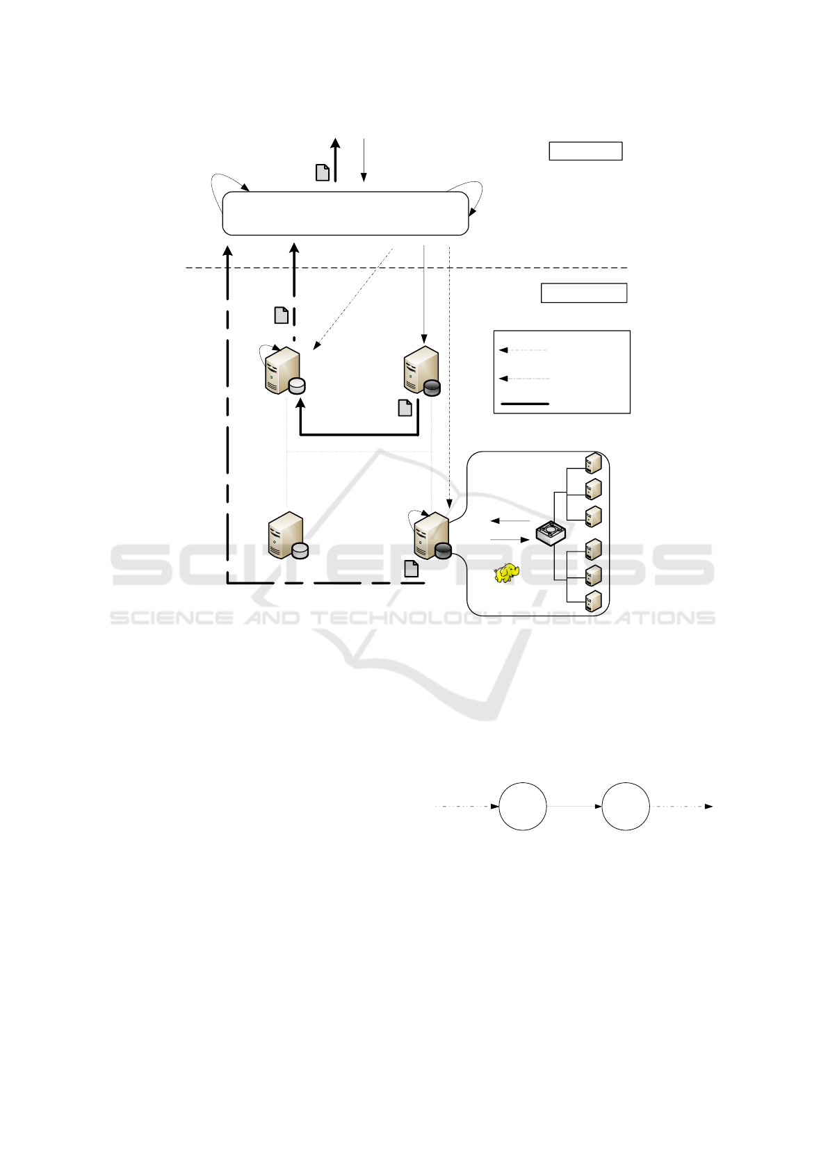
Top-Level Job

Output Data

Result

Local Hadoop Job

Top Level

Data Transfer

Top Level Manager

Execute Top-Level

MapTask

Reduce

Bottom Level

MoveData

Site1

Site3

Site2

Push Top-Level

Map Result

Site4

MapReduce

Generate TJEP

Figure 1: Job Execution Flow.

4 JOB SCHEDULING

Basically, the scheduling system’s strategy is to gen-

erate all the possible job execution paths for the ad-

dressed distributed computing context. Each gener-

ated path is characterized by a score, which is a func-

tion of the estimated job completion time (the shorter

the estimated completion time, the higher the score).

The calculation of the score for a given path con-

sists in the estimation of the path’s completion time.

The path exhibiting the lowest completion time (best

score) will be selected to enforce the job execution.

The job’s execution path representation is based

on a graph model where each graph node represents

either a Data Computing Element (site) or a Data

Transport Element (network link). Arcs between

nodes are used to represent the sequence of nodes in

an execution path (see Figure 2). A node representing

a computing element elaborates data, therefore it will

produce an output data ﬂow whose size is different

than that of the input data; a node representing a data

transport element just transports data, so for that node

the input data size and the output data are equal.

Node

j+1

DataSize

j-1, j

DataSize

j, j+i

DataSize

j+1, j+2

Throughput

j+1

Throughput

j+1

Figure 2: Nodes’ representation model.

Nodes are characterized by two parameters: the

compression factor β

app

, that is used to estimate the

data produced by a node, and the T hroughput, de-

ﬁned as the amount of data that the node is able to pro-

cess per time unit. The β

app

value for a Data Comput-

ing Element is equal to the ratio between the produced

output data and the input data to elaborate, while for

A LAHC-based Job Scheduling Strategy to Improve Big Data Processing in Geo-distributed Contexts

the Data Transport Elements it is equals to 1 because

there is no data computation occurring in a data trans-

fer. The T hroughput of a Data Computing Element is

rate at which the node is capable of producing data in

output, and of course it depends on the Site’s com-

puting capacity; for a Data Transport Elements the

Throughput just corresponds to the link capacity. A

generic node’s execution time is deﬁned as the ratio

between the input data size and the T hroughput of

the node.

In Figure 2, the label value of the arc connecting

node j −th to node ( j + 1) −th is given by:

DataSize

j, j+1

= DataSize

j−1, j

× β

(1)

A generic node j’s execution time is deﬁned as:

DataSize

j−1, j

T hroughput

(2)

Both the β and the Throughput are speciﬁc to the

job’s application that is going to be executed, and of

course they are not available at job submission time.

To estimate these parameters, we run the job on small-

sized samples of the data to elaborate. These test re-

sults allow us to build an application proﬁle made of

both the β and the T hroughput parameters, which will

be used as input of the top level job execution plan

process performed by the scheduler. The estimation

procedure is described in details in our previous work

(Cavallo et al., 2016b), where we proposed a study

of the job’s Application Proﬁle and analyzed the be-

havior of well know Map Reduce applications. The

number of the job’s potential execution paths depends

on the set of computing nodes, the links’ number and

capacity and the data size. A job’s execution path has

as many branches as the number of Map Reduce sub-

jobs that will be run. Every branch starts at the root

node (initial node) and ends at the Global Reducer’s

node. We deﬁne the execution time of a branch to be

the sum of the execution times of the nodes belonging

to the branch; the Global Reducer node’s execution

time is left out of this sum. The execution carried out

through branches are independent of each other’s, so

branches will have different execution times. In order

for the global reducing to start, all branches will have

to produce and move their results to the reducer Site.

The execution time of the Global Reducer is given

by the summation of the sizes of the data sets com-

ing from all the branches over the node’s estimated

throughput.

Let us show an example of execution path mod-

eling on a reference scenario. The example topology

(see Figure 3) is composed of four sites and a geo-

graphic network interconnecting the sites.

Let us suppose that a submitted top-level job

needs to process a 15 GB data set distributed among

Figure 3: Example Topology.

the Sites S

(5 GB) and S

(10 GB). In this example

we assume that the data block size (minimum com-

putable data unit) is 5 GB. Figure 4 shows the model

representing a potential execution path generated by

the Job Scheduler for the submitted job. The graph

model is a step-by-step representation of all the data

movements and data processing enforced to execute

the top level job. This execution path starts at the sites

, S

) where data reside at job submission time and

involves the movement of a 5GB data from S

to S

and from S

to S

. Then, three Hadoop sub-jobs will

be executed at S

, S

and S

respectively. Finally the

global reducing of the data produced by the Hadoop

sub-jobs will be performed at S

Figure 4: Graph modeling a potential execution path.

In the example, the branch at the bottom models

the elaboration of data that initially reside in node

, are map-reduced by node S

itself, and are ﬁnally

pushed to node S

(the Global Reducer) through the

links L

A 2

and L

A 3

. In the graph, only the L

A 2

node

is represented as it is slower than L

A 3

and will im-

pose its speed in the overall path S

→ L

A 2

→ R

→

A 3

→ S

. Similarly in the middle branch the data

resides in node S

, are moved to node S

through the

link L

, and are map-reduced by node S

itself. In

the top-most branch the data residing in node S

are

moved to node S

through link L

A 0

is slower

than L

A 1

), are map-reduced by node S

and are ﬁ-

nally pushed to node S

through link L

A 3

avail-

able bandwidth is less than L

A 1

bandwidth).

4.1 A Scalable Job Scheduling

Algorithm

The job scheduling algorithm’s task is to search for

an execution path which minimizes a given job’s ex-

ecution time. In our previous work (Cavallo et al.,

IoTBDS 2017 - 2nd International Conference on Internet of Things, Big Data and Security

2015) we proposed a job scheduling algorithm capa-

ble of generating all possible combinations of map-

pers and the related assigned data fragments by lever-

aging on the combinatorial theory. That approach’s

strategy was to explore the entire space of all poten-

tial execution paths and ﬁnd the one providing the best

(minimum) execution time. Unfortunately the num-

ber of potential paths to visit may be very large, if we

consider that many sites may be involved in the com-

putation and that the data sets targeted by a job might

be fragmented at any level of granularity. Of course,

the time to seek for the best execution plan consider-

ably increases with the number of fragments and the

number of network’s sites. That time may turn into

an unacceptable overhead that would affect the per-

formance of the overall job. If on the one hand such

an approach guarantees for the optimal solution, on

the other one it is not scalable.

In order to get over the scalability problem, in

this work we propose a new approach that searches

for a good (not necessarily the best) job execution

plan which still is capable of providing an accept-

able execution time for the job. Let us consider the

whole job’s makespan divided into two phases: a pre-

processing phase, during which the job execution plan

is deﬁned, and a processing phase, that is when the

real execution is enforced. The new approach aims

to keep the pre-processing phase as short as possible,

though it may cause a time stretch during the process-

ing phase. We will prove that, despite the time stretch

of the job’s execution, the overall job’s makespan will

beneﬁt.

Well known and common optimization algorithms

follow an approach based on a heuristic search

paradigm known as the one-point iterative search.

One point search algorithms are relatively simple

in implementation, computationally inexpensive and

quite effective for large scale problems. In general,

a solution search starts by generating a random initial

solution and exploring the nearby area. The neighbor-

ing candidate can be accepted or rejected according to

a given acceptance condition, which is usually based

on an evaluation of a cost functions. If it is accepted,

then it serves as the current solution for the next iter-

ation and the search ends when no further improve-

ment is possible. Several methodologies have been

introduced in the literature for accepting candidates

with worse cost function scores. In many one-point

search algorithms, this mechanism is based on a so

called cooling schedule (CS) (Hajek, 1988). A weak

point of the cooling schedule is that its optimal form

is problem-dependent. Moreover, it is difﬁcult to ﬁnd

this optimal cooling schedule manually.

The job’s execution path generation and evalua-

tion, which represent our optimization problem, are

strictly dependent on the physical context where the

data to process are distributed. An optimization al-

gorithm based on the cooling schedule mechanism

would very likely not ﬁt our purpose. Finding a con-

trol parameter that is good for any variation of the

physical context and in any scenario is not an easy

task; and if it is set up incorrectly, the optimization

algorithm fail shortening the search time. As this pa-

rameter is problem dependent, its ﬁne-tuning would

always require preliminary experiments. Unfortu-

nately, such preliminary study can lead to additional

processing overhead. Based on these considerations,

we have discarded optimization algorithms which en-

vision a phase of cooling schedule.

The optimization algorithm we propose to use in

order to seek for a job execution plan is the Late Ac-

ceptance Hill Climbing (LAHC) (Burke and Bykov,

2008). The LAHC is an one-point iterative search al-

gorithm which starts from a randomly generated ini-

tial solution and, at each iteration, evaluates a new

candidate solution. The LAHC maintains a ﬁxed-

length list of the previously computed values of the

cost function. The candidate solution’s cost is com-

pared with the last element of the list: if it is not

worse, it is accepted. After the acceptance procedure,

the cost of the current solution is added on top of the

list and the last element of the list is removed. This

method allows some worsening moves which may

prolong the search time but, at the same time, helps

avoiding local minima. The LAHC approach is sim-

ple, easy to implement and yet is an effective search

procedure. This algorithm depends on just the input

parameter L, representing the length of the list. It is

possible to make the processing time of LAHC inde-

pendent of the length of the list by eliminating the

shifting of the whole list at each iteration.

The search procedure carried out by the LAHC is

better detailed in reported in the Algorithm 1 listing.

The LAHC algorithm ﬁrst generates an initial solu-

tion which consists of a random assignment of data

blocks to mappers. The resulting graph represents the

execution path. The evaluated cost for this execution

path is the current solution and it is added to the list.

At each iteration, the algorithm evaluates a new can-

didate (assignment of data blocks and mappers nodes)

and calculates the cost for the related execution path.

The candidate cost is compared with the last element

of the list and, if not worse, is accepted as the new

current solution and added on top of the list. This

procedure will continue until the reach of a stopping

condition. The last found solution will be chosen as

the execution path to enforce.

In the next section we compare the LAHC algo-

A LAHC-based Job Scheduling Strategy to Improve Big Data Processing in Geo-distributed Contexts

Algorithm 1: Late Acceptance Hill Climbing

algorithm applied to the problem of job execu-

tion time minimization.

Produce random job execution path (initial

solution) s

Calculate initial solution’s cost function C(s)

Specify the list length L

begin

for k ∈ {0..L − 1} do

C(k) ← C(s)

end

Assign the initial number of iteration I ← 0

repeat

Produce a new job execution path (new

candidate solution) s∗

Calculate its cost function C(s∗)

v ← I mod L

if C(s∗) ≤ C

then

accept candidate (s ← s∗)

end

else

reject candidate (s ← s)

end

Add cost value on top of the list

← C(s)

Increment the number of iteration

I ← I + 1

until a chosen stopping condition;

end

rithm with the scheduler’s algorithm based on a com-

binatorial approach. Objective of the comparison is

to prove that the newly introduced algorithm scales

better and is even capable of producing better perfor-

mance in terms of reduced job makespan.

5 EXPERIMENTS

In this section we report the result of a comparison test

we ran to measure the increase of performance that

the new job scheduling algorithm is able to provide

with respect to the combinatorial algorithm discussed

in (Cavallo et al., 2016b). Main objective of the test is

to study the scalability of the two algorithms. To this

purpose, we designed some conﬁgurations - that are

meant to represent different scenarios - by tuning up

the following parameters: the number of Sites popu-

lating the geographic context, the network topology

interconnecting the Sites and number of data blocks

distributed among the Sites.

The experiments were done by simulating the ex-

ecution of a job with given β

app

and T hroughput.

=20GFLOPS

1122

=10MB/s

113

=10MB/s

111

= 10MB/s

225

=10MB/s

224

= 10MB/s

112

=10MB/s

=20GFLOPS

Figure 5: Network topology with 5 Sites.

Speciﬁcally, we considered a sample Job for which

a β

app

value of 0.5 was estimated. The results that we

show is an average evaluated over 10 runs per conﬁg-

uration.

In the considered scenarios, each node is equipped

with a 20 GFLOPS of computing power and each

network’s link has a 10 MB/s bandwidth. Further,

the size of every data block is set to 500MB. As for

the LAHC algorithm, we also ran several preliminary

tests in order to ﬁnd a proper list’s size value. From

those tests, we observed that this parameter does not

have a substantial impact on the search of the execu-

tion path by the LAHC, neither it impairs the over-

all LAHC performance. For the test purpose, it was

arbitrarily set it to 100. Moreover, we set the stop-

ping condition for the LAHC to 10 seconds, meaning

that the algorithm stops its search after 10 seconds of

computation. This parameter’s value, again, comes

from preliminary tests that were run in order to ﬁgure

out what an acceptable stopping condition would be.

From those tests we observed that pushing that pa-

rameter to higher values did not bring any substantial

beneﬁt in the search of the job execution path. Fi-

nally, the two scheduling algorithms were both run on

the same physical computing node, which is equipped

with an i7 CPU architecture and a 16 GB RAM.

A ﬁrst battery of tests was run on a network topol-

ogy made up of ﬁve Sites interconnected to each

other’s in the way that is shown in Figure 5. From

this topology, ﬁve different conﬁgurations were de-

rived by considering the number of data blocks set to

5, 10, 20, 40 and 80 respectively. A second battery of

tests was then run for another network topology that

was obtained by just adding a new Site to the former

topology (the new Site was attached to switch R

just

in between S

and S

. That, of course, made things

more complicated since the number of combinations

of all possible job execution path increases. As for

this network topology, the same data block conﬁgura-

tions were considered. Unfortunately, we had to stop

the 80 data-block test as it took more than two days

IoTBDS 2017 - 2nd International Conference on Internet of Things, Big Data and Security

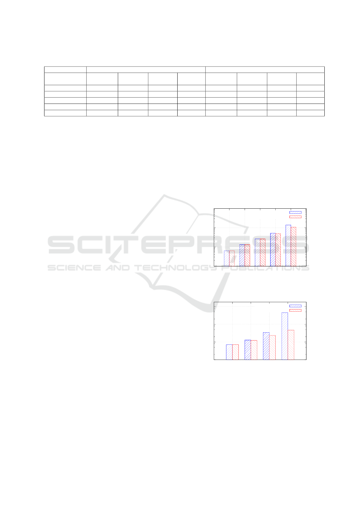
Table 1: KPIs measured in the 5-node network topology.

Combinatorial LAHC

# of DataBlocks

Scheduling

Time [sec]

Execution

Time [sec]

Makespan

[sec]

Overhead

[%]

Scheduling

Time [sec]

Execution

Time [sec]

Makespan

[sec]

Overhead

[%]

5 1.49 6375 6376 0.02 10.32 6375 6385 0.16

10 5.63 13250 13256 0.04 10.01 13250 13260 0.07

20 256.02 26250 26506.02 0.96 10.01 26250 26260 0.038

40 3215.42 49000 52215.42 6.15 10.01 49750 49760 0.020

80 42280 96750 139030 30.41 10.32 106500 106510 0.0097

for the combinatorial algorithm to run without even

ﬁnishing.

The KPI that is put under observation is the job

makespan. That KPI is further decomposed in two

sub-KPIs: the job scheduling time and the job exe-

cution time. Throughout the tests, the two sub-KPIs

were measured. Results of the ﬁrst battery of tests are

shown in Table 1. In the table, for each algorithm, we

report the following measures: scheduling time, exe-

cution time, makespan (which is the sum of the pre-

vious two measures) and the overhead (the percent-

age of the scheduling time over the makespan). The

reader may notice that in the cases of 5 and 10 data

blocks respectively the combinatorial algorithm out-

performs the LAHC in terms of makespan. In those

cases, the LAHC managed to ﬁnd the global optimum

(we remind that the combinatorial always ﬁnds the

optimum) but the LAHC overhead is higher than that

of the combinatorial (which is capable of ﬁnding the

solution in much less than 10 seconds). In the case of

20 data blocks, the LAHC is still able to ﬁnd a global

optimum, so the performance of the two algorithm

terms of execution time are equal. But in this case

the combinatorial took more than 200 seconds to ﬁnd

the solution, while the scheduling time for the LAHC

is always ten seconds long. So the LAHC slightly out-

performs the combinatorial in the makespan. Finally,

in the cases of 40 and 80 data blocks the LAHC ﬁnds

a just local optimum (the LAHC’s execution time is

lower than the combinatorial’s). In spite of that, being

the scheduling time of the combinatorial extremely

long, in the makespan comparison the LAHC once

more outperforms the combinatorial.

In Figure 6 we have reported the two execution

paths found by the two algorithms in the case of 40

data blocks. While the combinatorial’s is the best pos-

sible path and the LAHC’s is only a local optimum,

the two paths look very much alike. The only differ-

ence, which is highlighted in the red boxes, concerns

the computation of the data residing in Site S

. While

the LAHC schedules the computation of the data on

the Site S

itself, the combinatorial manages to bal-

ance to computation between Site S

and Site S

, thus

speeding up the overall execution time.

Results of the second battery of tests are shown

in Table 2. The reader will notice that in the new net-

work topology, which is a little more complex than the

previous one, the combinatorials has some scalabil-

ity issues even with a relatively simplex data conﬁg-

uration (for 10 data blocks, the scheduling time takes

more than 500 seconds. In the cases of 20 and 40

blocks respectively, the LAHC conﬁrms to be the best

as it is capable of ﬁnding very good execution paths

(though not the best) in a very short scheduling time.

1000

10000

100000

1x10

5 10 20 40 80

Makespan [sec]

# of Data Blocks

Combinatorial

LAHC

Figure 7: Makespan in the 5-node network topology.

1000

10000

100000

1x10

5 10 20 40

Makespan [sec]

# of Data Blocks

Combinatorial

LAHC

Figure 8: Makespan in the 6-node network topology.

In Figures 7 and 8 we reported a graphical rep-

resentation of the makespan performance of the two

algorithms. In the graph, for the ease of representa-

tion, the values in y-axis are reported in a logarithmic

scale. The ﬁnal consideration that we draw is that the

combinatorial algorithm is extremely poor in terms of

scalability. In fact, the performance will degrade sig-

A LAHC-based Job Scheduling Strategy to Improve Big Data Processing in Geo-distributed Contexts

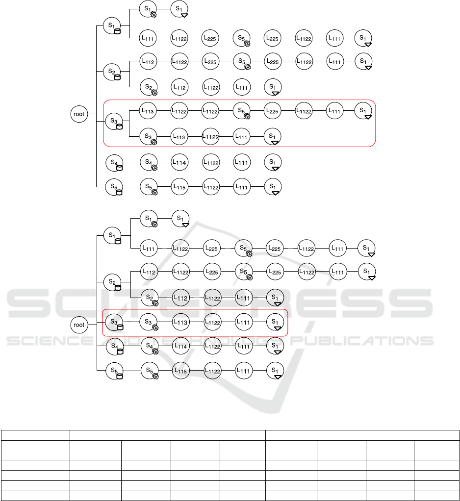
(a)

(b)

Figure 6: Execution paths in the 5-node network topology and the 40 data-blocks conﬁguration: a) combinatorial; b) LAHC.

Table 2: KPIs measured in the 6-node network topology.

Combinatorial LAHC

# of DataBlocks

Scheduling

Time [sec]

Execution

Time [sec]

Makespan

[sec]

Overhead

[%]

Scheduling

Time [sec]

Execution

Time [sec]

Makespan

[sec]

Overhead

[%]

5 1.87 7125 7126 0.03 10.36 7125 7135 0.14

10 594 12250 12844 4.62 10.13 12250 12260 0.083

20 10795.30 23500 34295.3 31.48 10.02 23500 23510 0.043

40 404980.31 44350 449330.31 90.13 10.10 47000 47010 0.021

niﬁcantly as the number of data blocks grows. The

LAHC solution was proved to scale very well. De-

spite the solutions it ﬁnds are local optima, even for

very complex scenarios they are very close to the

global optima found by the combinatorial.

6 CONCLUSION

The gradual increase in the information daily pro-

duced by devices connected to the Internet, combined

with the enormous data stores found in traditional

databases, has led to the deﬁnition of the Big Data

concept. This work aims to make big data process-

IoTBDS 2017 - 2nd International Conference on Internet of Things, Big Data and Security

100

ing more efﬁcient in geo-distributed computing envi-

ronments, i.e., environments where data to be com-

puted are scattered among data centers which are ge-

ographically distant. In this paper we describe a job

scheduling solution based on the Late Acceptance

Hill-Climbing (LAHC) algorithm, that allows to ﬁnd

a sub-optimal job execution plan in a very limited

scheduling time. For our purposes, several scenarios

were designed that reproduce many geographical dis-

tributed computing contexts. We compared the per-

formance produced by the LAHC with that of a com-

binatorial algorithm we had proposed in a previous

paper. Results show that the LAHC scales very well

in very complex scenarios and always guarantees a

job makespan that is shorter than the one provided by

the combinatorial algorithm. Encouraged by these re-

sults, our future works will focus on ensuring a job

fair scheduling and an optimum exploitation of the

computing resources in multi-job scenarios.

REFERENCES

Burke, E. K. and Bykov, Y. (2008). A late acceptance strat-

egy in hill-climbing for examination timetabling prob-

lems. In Proceedings of the conference on the Practice

and Theory of Automated Timetabling(PATAT).

Cavallo, M., Cusm

a, L., Di Modica, G., Polito, C., and

Tomarchio, O. (2015). A Scheduling Strategy to Run

Hadoop Jobs on Geodistributed Data. In Advances in

Service-Oriented and Cloud Computing: Workshops

of ESOCC 2015, Taormina, Italy, September 15-17,

2015, Revised Selected Papers, volume 567 of CCIS,

pages 5–19. Springer.

Cavallo, M., Cusm

a, L., Di Modica, G., Polito, C., and

Tomarchio, O. (2016a). A Hadoop based Framework

to Process Geo-distributed Big Data. In Proceedings

of the 6th International Conference on Cloud Com-

puting and Services Science (CLOSER 2016), pages

178–185, Rome (Italy).

Cavallo, M., Di Modica, G., Polito, C., and Tomar-

chio, O. (2016b). Application Proﬁling in Hierarchi-

cal Hadoop for Geo-distributed Computing Environ-

ments. In IEEE Symposium on Computers and Com-

munications (ISCC 2016), Messina (Italy).

Hajek, B. (1988). Cooling schedules for optimal annealing.

Mathematics of Operations Research, 13(2):311–329.

Heintz, B., Chandra, A., Sitaraman, R., and Weissman, J.

(2014). End-to-end Optimization for Geo-Distributed

MapReduce. IEEE Transactions on Cloud Comput-

ing, 4(3):293–306.

Jayalath, C., Stephen, J., and Eugster, P. (2014). From

the Cloud to the Atmosphere: Running MapReduce

across Data Centers. IEEE Transactions on Comput-

ers, 63(1):74–87.

Kim, S., Won, J., Han, H., Eom, H., and Yeom, H. Y.

(2011). Improving Hadoop Performance in Intercloud

Environments. SIGMETRICS Perform. Eval. Rev.,

39(3):107–109.

Luo, Y., Guo, Z., Sun, Y., Plale, B., Qiu, J., and Li, W. W.

(2011). A Hierarchical Framework for Cross-domain

MapReduce Execution. In Proceedings of the Second

International Workshop on Emerging Computational

Methods for the Life Sciences, ECMLS ’11, pages 15–

22.

Mattess, M., Calheiros, R. N., and Buyya, R. (2013). Scal-

ing MapReduce Applications Across Hybrid Clouds

to Meet Soft Deadlines. In Proceedings of the 2013

IEEE 27th International Conference on Advanced In-

formation Networking and Applications, AINA ’13,

pages 629–636.

Miorandi, D., Sicari, S., Pellegrini, F. D., and Chlamtac, I.

(2012). Internet of things: Vision, applications and

research challenges. Ad Hoc Networks, 10(7):1497 –

1516.

Yang, H., Dasdan, A., Hsiao, R., and Parker, D. S. (2007).

Map-reduce-merge: Simpliﬁed relational data pro-

cessing on large clusters. In Proceedings of the 2007

ACM SIGMOD International Conference on Manage-

ment of Data, SIGMOD ’07, pages 1029–1040.

Zhang, Q., Liu, L., Lee, K., Zhou, Y., Singh, A.,

Mandagere, N., Gopisetty, S., and Alatorre, G. (2014).

Improving Hadoop Service Provisioning in a Geo-

graphically Distributed Cloud. In Cloud Computing

(CLOUD), 2014 IEEE 7th International Conference

on, pages 432–439.

A LAHC-based Job Scheduling Strategy to Improve Big Data Processing in Geo-distributed Contexts

101