Energy Efficiency of a Multizone Office Building:
MPC-based Control and Simscape Modelling
Farah Gabsi
1
, Frederic Hamelin
1
, Remi Pannequin
1
and Mohamed Chaabane
2
1
Centre de Recherche en Automatique de Nancy - University of Lorraine, Vandoeuvre-les-Nancy, France
2
Laboratoire des Sciences et Techniques de l’Automatique et de l’informatique industrielle - ENIS, Sfax, Tunisia
Keywords:
Energy-efficient Buildings, Simscape
TM
Models, Model Predictive Control, Multi-room Building Model.
Abstract:
This paper deals with the problem of modelling and controlling a multi-zone office building to ensure its
thermal comfort by an optimal and cost effective management of the energy consumption. A thermal behaviour
analysis of the building is carried out using the Simscape
TM
library in MATLAB/Simulink
R

environment
that leads to a multi-model representation. Based on this modelling, the Yalmip toolbox in the MATLAB
programming environment or an iterative optimization algorithm can be used to solve the control optimisation
problem. The design of a model predictive control associated with a wise choice of the cost function makes it
possible to obtain in simulation substantial energy benefits.
1 INTRODUCTION
Over the last years, a large number of researchers
have been interested in controlling strategies for en-
ergy saving of buildings (Scherer et al., 2014), (Atam
and Helsen, 2016). Indeed, the construction sector,
especially electrical energy, is the largest energy con-
sumer. It represents approximately 40% of the total
energy consumption between all sectors of the econ-
omy in France and in the US (Agbi, 2014). One of
possible approaches to reduce energy consumption in
buildings is to use advanced control tools to effec-
tively monitor all the building actuators to ensure its
hygrothermal comfort (Goyal et al., 2013), (Privara
et al., 2011).
In this paper, a thorough methodology of mod-
elling/controlling a building part is proposed to ensure
the thermal comfort of its inhabitants while minimiz-
ing energy consumption. It uses the Simscape
TM
tool-
boxes to model the thermal behaviour of the build-
ing (Lapusan et al., 2016), and an iterative algorithm
(or Yalmip (Lofberg, 2004)) to solve the optimization
problem related to the synthesis of a predictive con-
trol. The applied target is the “Eco-safe” platform
(CRAN Nancy, France) that fits in a global context
of smart home. The developed Simscape
TM
model is
based on a physical description of the building. This
approach allows the description of the system as a
physical structure rather than by abstract mathemat-
ical equations. Furthermore, the differential equa-
tions that describe the thermal behaviour of the sys-
tem can be directly generated from the Simscape
TM
model. This modelling step in the form of a state-
space representation is essential for the development
of a predictive control model (MPC) (Camacho and
Bordons, 2007). This type of control is favoured be-
cause it has the advantage of taking into account the
disturbance predictions that greatly influence the inte-
rior comfort of a building (outside temperature, sun-
shine, occupations of parts) while anticipating their
effects (Ma et al., 2011), (Oldewurtel et al., 2012),
(Privara et al., 2011). Knowing that each control ac-
tion is associated with a different state-space model of
the system, the predictive control used is considered
as a hybrid type (Le et al., 2014). In view of the con-
trol objectives, the associated optimization criterion
is defined to integrate the energy cost of each actuator
in kWh, the resolution of the optimization problem is
executed using the Yalmip tool of Matlab or an itera-
tive algorithm for important prediction horizon.
The first part of this work is focused on the thermal
modelling of a set of building parts because few works
have been interested in this issue. The validation of
the model and the control will be conducted on the
“Eco-safe” platform. Next a model predictive control
is put in order to ensure the thermal comfort of the
rooms of the platform with a minimum of energy con-
sumption. Tests of simulation with various scenarios
were developed to exhibit the energy benefits.
Gabsi, F., Hamelin, F., Pannequin, R. and Chaabane, M.
Energy Efficiency of a Multizone Office Building: MPC-based Control and Simscape Modelling.
DOI: 10.5220/0006305002270234
In Proceedings of the 6th International Conference on Smart Cities and Green ICT Systems (SMARTGREENS 2017), pages 227-234
ISBN: 978-989-758-241-7
Copyright © 2017 by SCITEPRESS – Science and Technology Publications, Lda. All rights reserved
227

2 PLATFORM DESCRIPTION
The “Eco-safe” platform consists of 6 rooms and a
corridor (Figure 1). The rooms are equipped with sen-
sors and actuators to model their thermal behaviour
and control their comfort. Regarding the area, the
platform is characterized by two main activity rooms:
“a room of research and development” (R&D,
1
) of
51m
2
and a piece of applications
5
 of 34m
2
. Four
other rooms, 17m
2
each, allow to store tools and var-
ious materials (parts
2
+
4
) or to have an estimate
of the rooms temperature located in the upper and
lower floors (
3
+
6
), because with the same neutral
behaviour. The platform consists of heterogeneous
equipment architecture such as the sensors needed for
the modelling of its thermal response, the equipment
contributing to the thermal comfort of the rooms and
a weather station that integrates several sensors. To
ensure the thermal comfort of this platform by imple-
menting a predictive control based on the minimiza-
tion of energy consumption, it is necessary to deter-
mine a model for the thermal behaviour of the plat-
form. The following paragraph provides an answer to
this objective through the definition of a simulator.
Figure 1: The “Eco-safe” deck plans.
3 THERMAL MODELLING OF
THE PLATFORM
The simplified physical model we aim to establish has
the role to predict the thermal behaviour of the whole
platform. The latter is decomposed piece by piece
taking into account their orientation in order to fur-
ther simulate the influence of the solar radiation. Each
room consists of different elements (walls, ceiling,
floor, windows), some of which benefit from some
solar energy inputs. The temperature of the R&D
room, (
1
) and applications (
5
) is also influenced
by a main source of energy which is a reversible heat
pump to produce the heat and cold. In addition, air
flow is provided between these same rooms through
two controlled mechanical ventilation (CMV). Over-
all, the energy balance for each of the rooms can be
translated by the following equation:
C
int
dT
int
dt
= f
ext
(T
ext
,T
int
) +
n
∑
i=1
f
i
(T
int
,T
int,i
)
+θ
occupancy
+ θ
energy
(1)
with:
• C
int
: heat capacity (J/K) of the considered room;
• T
int
, T
ext
and T
int,i
: temperature (K) of the consid-
ered room, of outside and of the adjacent rooms;
• θ
energy
and θ
occupancy
: energy contributions (W )
and heat generated by the inhabitants of the room;
• f
ext
(T
ext
,T
int
) and f
i
(T
int
,T
int,i
): functions reflect-
ing the thermal behaviour of interfaces between
the room and the outside or adjacent rooms.
In order to establish the complete thermal model
of the “Eco-safe” platform, we use a physical ap-
proach based on the Simscape
TM
tool (Lapusan et al.,
2016) in the environment Simulink
R

. The global
model of the platform is the result of the integration of
all room models. Each room includes walls and win-
dows that are interacting with the external environ-
ment and neighbouring rooms by each mode of heat
transfer. While this issue is the subject of the section
that follows, the energy sources influencing the room
thermodynamics are modelled in the last paragraph.
3.1 Thermal Modelling of a Room
The room model is developed using the thermal el-
ements library of Simscape
TM
. If a correspondence
is established between the flow of heat and electric
power as well as between the temperature and the
potential difference, it is conventional to establish
thermoelectric analogies (Achterbosch et al., 1985).
This analogy will be used in the transcript of the
Simscape
TM
model of the platform to a state-space
model.
3.1.1 Models of a Wall and a Set of Windows
Wall: The thermal equilibrium is established tak-
ing into account the convective exchange between the
wall and the air that surrounds it on each side. In-
side the wall, the heat is transferred through con-
duction phenomenon. The wall model developed on
Simscape
TM
model is presented in Figure 2a, in which
it is assumed that the wall is the interface between the
inside of a room and the outside air. By electrical
analogy, the wall can also be described by a 2R1C
model (2 resistors and 1 capacitor) and schematically
represented in Figure 2b, which presents the follow-
ing notations:
SMARTGREENS 2017 - 6th International Conference on Smart Cities and Green ICT Systems
228

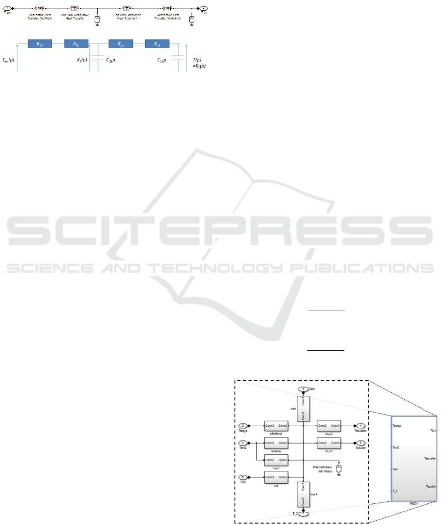
• X
1
(p), X
2
(p), T
ext
(p): temperature (K) of the
room, in the middle of the wall and of outside;
• (R
11
, R
41
) and (R
21
, R
31
): thermal resistances
(K/W ) of convection and conduction;
• C
11
, C
21
: heat thermal capacities (J/K) of the
room and of the exterior wall.
Figure 2: Model of a wall (a) by Simscape
TM
(b) by electri-
cal analogy.
Set of windows: To model the thermal behaviour of
all windows in a room, we assumed that it was iden-
tical to consider a single window of equivalent sur-
face. Knowing that the windows in the rooms are all
double glazed, their modelling requires to take into
account not only the surface/superficial resistance of
inside and outside exchange (transfer by convection/
convective transfer) but also transfers by conduction
within the two glass panes and the air space between
them (see Figure 3a). By analogy, a 4R3C model is
used to determine the associated state-space represen-
tation (see Figure 3b). with:
• X
0
1
(p), X
0
2
(p), X
0
3
(p) and X
0
4
(p): temperature (K)
of the room and in the middle of the inner glass,
of the air space and of the outer glass;
• (R
12
, R
82
) and (R
22
, R
32
,..., R
62
, R
72
): thermal
resistances (K/W ) of convection and conduction;
• C
22
, C
32
, C
42
: heat thermal capacities (J/K) of the
glass and of the air space/blade;
The state-space representations of a wall and of a set
of windows are then obtained by the application of
Millman’s theorem.
3.1.2 Models of a Room and “Eco-safe”
Platform
Room: A room being made up of several walls, a
slab, a ceiling (whose thermal behaviour is similar
to that of a wall in our case) and possible windows,
the one-room model is obtained by the integration of
the models of each of these elements within a unique
state-space representation. Considering the R&D
room (
1
) of the platform “Eco-safe” represented in
Figure 4, the state-space model thus obtained is of
order 11 (5 adjacent walls (order 1) + 1 ceiling (order
1) + 1 ground (order 1) + 1 set of windows (order 3)
+ heat capacity of the room (order 1)).
“Eco-safe” Platform: The platform is modelled by
a set of rooms delimited by the walls that are in ther-
mal contact with the outside environment and neigh-
bouring rooms. Applying the same technique of mod-
elling than for room
1
, we get a state-space represen-
tation of order 72 to simulate the thermal behaviour of
the platform. In this model, the temperature values of
the upper and lower floors are considered to be iden-
tical to those of the reference rooms (
3
+
6
).
3.2 Modelling of Energy Sources
The most important elements that produce the heat or
cold inside the building are the reversible heat pump,
the ventilation system and sun radiation. These differ-
ent equipments/contributions of energy are modelled
in this paragraph to be integrated in the simulator. The
model also takes into account the effect of the people
inside the platform and that of different electrical ap-
pliances that generate heat.
3.2.1 CMV
The CMV is used to circulate the air between rooms
1
 and
5
 (see Figure 1). It is assumed that the air
taken in the ‘source’ room is replaced by the outside
air through the openings at the level of the windows.
On the other hand, air received by the ‘destination’
room replaces a part of its air that is equally displaced
through the openings at the level of the windows. If
we take the example that the air flows from room
5

to room
1
, the energy flows generated by the CMV
are at the level of the ‘source’ room:
φ
CMV 1
(t) =
ρc
1
D
CMV
3600
(T
ext
(t) − T
5

(t)) (2)
and at the level of the ‘destination’ room:
φ
CMV 2
(t) =
ρc
1
D
CMV
3600
(T
5

(t) − T
1

(t)) (3)
Figure 4: Model Simscape
TM
exhibit R&D (
1
).
Energy Efficiency of a Multizone Office Building: MPC-based Control and Simscape Modelling
229

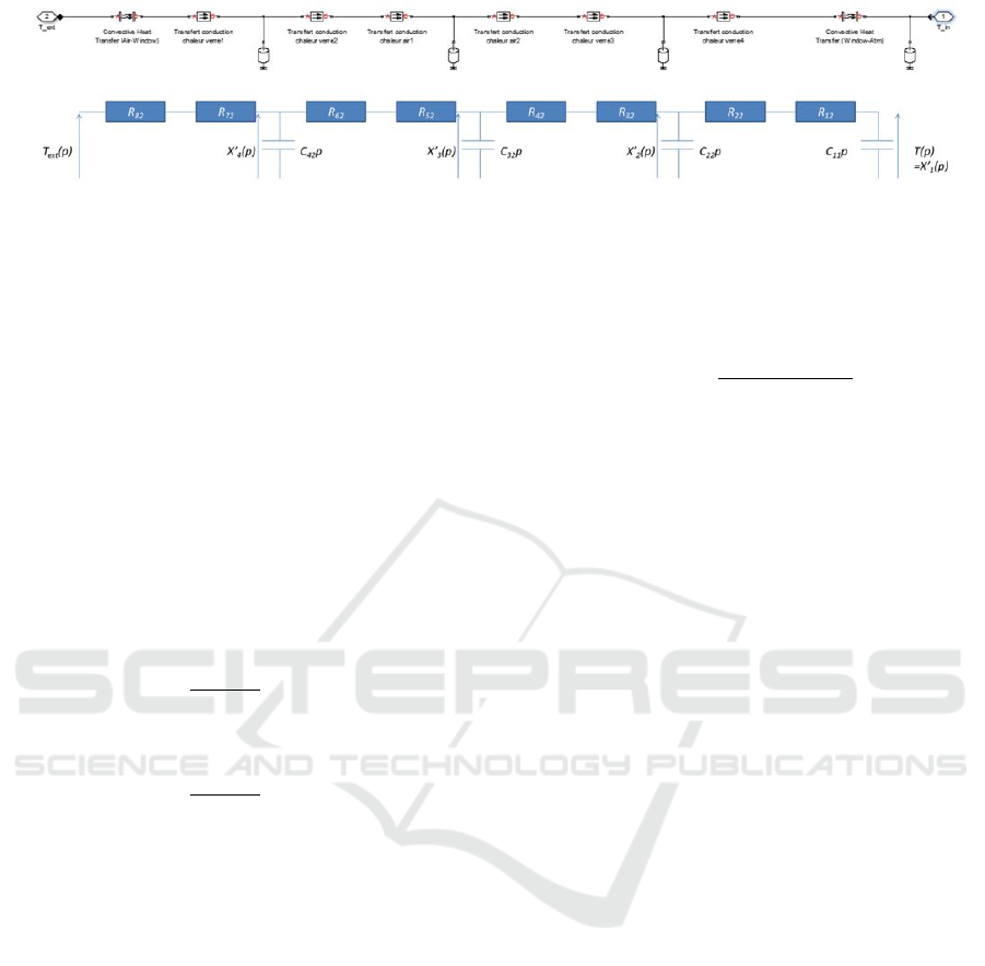
Figure 3: Model of a set of windows (a) by Simscape
TM
(b) par electrical analogy.
with c
1
= 1005.4 J/kg/K the specific heat of air ; ρ =
1.204 kg/m
3
the density of air ; D
CMV
= 150 m
3
/h the
air flow of the CMV ; (T
ext
, T
1

, T
5

) the tempera-
tures (K) of outside atmosphere, of rooms
1
 and
5
.
3.2.2 Reversible Heat Pump (HP)
A heat pump is a thermodynamic device that allows
capturing heat from outdoor air and transmitting it in-
side the building. Being reversible, the HP air – water
of the platform is capable of providing air condition-
ing in the summer. It starts running in heating mode
in the order of 312K and 290K into cooling mode.
Essentially, and without taking into account the tran-
sitional aspects, the equation translating this energy
flow is in the heating mode:
φ
HP1
(t) =
ρc
1
D
HP
3600
(312 − T
i
(t)) (4)
and in air conditioning mode:
φ
HP2
(t) =
ρc
1
D
HP
3600
(290 − T
i
(t)) (5)
with D
HP
= 5000 m
3
/h the air flow of the HP and T
i
the room temperature (K) in which the HP is used.
3.2.3 Modelling of the Occupation
Each individual has a sensible heat (by his/her body
at 37
◦
C) and a latent heat (by his/her production of
steam in breathing and perspiration). Different values
are given in the literature (ASHRAE, 2013). A person
generates about 100W . By multiplying this value by
the number of people in a room, we get the energy
released by them.
3.2.4 Inputs of Energy by Solar Radiation
The sun provides heat that greatly influences the tem-
perature within the platform rooms. The estimated
brought solar energy requires to instantly follow the
positioning of the sun and to take into account the ra-
diation so that diffuse direct. In order to understand
the calculations to quantify the global radiation, it is
important to define not only the various solar compo-
nents, but also the different angles used for calcula-
tions (Antonic, 1998). The energy related to the direct
radiation is such that:
S = 1230exp(−
1
3.8sin(h + 1.6)
)cos(β) (6)
where h is the height of the sun and β is the angle
between the normal to the windows and the solar rays.
They depend on the the latitude, the hour angle, the
solar declination and the solar azimuth. As for the
energy associated to the diffused radiation energy, it
is calculated by the relationship :
D = 125(sin(h)
0.4
)((1 + cos(i))/2)
+alb(((1 + cos(i))/2)(1080(sin(h)
1.22
) (7)
−125(sin(h)
0.4
)))sin(h) +125(sin(h)
0.4
)(1 −sin(h))
where alb = 0.2 is the albedo and i = 90 corresponds
to the inclination of the windows according to the hor-
izontal.
3.3 Simulation Results
The simulator is implemented by integrating the set
of energy sources described in the previous paragraph
to the Simscape
TM
model of the “Eco-safe” platform.
The associated state-space representation is deter-
mined by adding these different energy sources on the
equivalent electrical schemas/diagrams in terms of the
correspondence between a heat flow and an electric
current. The use of the CMV or HP has the effect of
changing the state-space model of the system. Con-
sidering different scenarios of following control, it is
possible to define 6 state-space models of the plat-
form:
• Scenario 0: no action on the system,
• Scenario 1: CMV switched room
5
 to
1
,
• Scenario 2: CMV switched room
1
 to
5
,
• Scenario 3: HP operated in the room
1
,
• Scenario 4: HP operated in the room
5
,
• Scenario 5: 2 HP operated in rooms
1
 and
5
.
SMARTGREENS 2017 - 6th International Conference on Smart Cities and Green ICT Systems
230

For simulation, continuous time models are finally
discretized with a 5-mn sampling period. They be-
come:

x(k + 1) = A
sim
i
x(k) + B
sim
i
d(k)
y(k) = C
sim
x(k)
(8)
with:
• i ∈ {0,..., 5}: the type of implemented control on
the system identically to the number of scenario;
• A
sim
i
and B
sim
i
: state and input matrices associated
with the number of scenario; C
sim
: output matrix;
• x(k) ∈ R
72
: state vector grouping all temperatures
of walls, windows and rooms of the platform.
• d(k) =

T
ext,k
Occ
k
Sol
west
k
Sol
east
k
T
HP,k

T
;
• y(k) =

T
1
,k
T
2
,k
T
corridor,k
T
4
,k
T
5
,k

T
;
• T
ext,k
: outside temperature (K);
• Occ
k
: energy brought by occupants of room
1
;
• Sol
west
k
and Sol
east
k
: energy provided by solar ra-
diation for rooms
1
,
2
,
3
 and
4
,
5
,
6
 resp.;
• T
HP,k
: temperature of the air forced through the
HP, T
HP,k
=290K (cold mode) or 312K (hot mode).
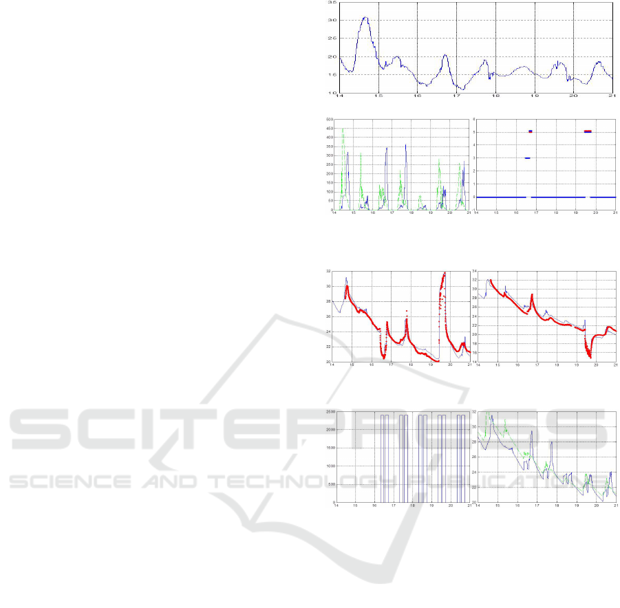
Parameters R
i j
and C
i j
of the simulator were calcu-
lated from the nature and characteristics of the dif-
ferent materials used in the wall dividers, walls and
windows of the platform. They have been adjusted
from the temperature curves actually observed on the
system. According to figures 7a and 7b, it appears
that the profiles of actual and estimated temperature
values are found to be very similar. The simulated
curves were generated according to the different sce-
narios of control represented in Figure 6b and from
the entries T
ext,k
(Figure 5), Sol
west
k
and Sol
east
k
(Fig-
ure 6a), which are the data issued from the meteorol-
ogy station over the period 14/09/2016 - 20/09/2016.
Figure 8b represents the temperature estimated by the
simulator within rooms
1
 and
5
 in scenario 0. In ad-
dition to the previous inputs, the energy released from
occupancy Occ
k
(figure 8a) is also considered. The
latter represents approximatively the energy genera-
ted by 24 people in room
1
 assuming their presence
all the open days from 8h to 12h and from 14h to 18h.
The following paragraph aims to implement a con-
trol law on the platform, which is capable of ensuring
thermal comfort in the occupied rooms while mini-
mizing energy consumption. A predictive control is
used on the basis of the simulator of the platform.
4 PREDICTIVE CONTROL
The principle of the predictive control (Camacho and
Bordons, 2007) is to optimize a cost function allow-
ing to describe the aim of control over a finite time
Figure 5: Outside temperature (14/09 - 20/09/2016).
Figure 6: (a) Solar energy (W ) Sol
west
k
(green) and Sol
east
k
(blue), (b) Control scenarios: HP in cold mode on 16/09 and
hot mode on 19/09 in room
1
 (inversely for room
5
).
Figure 7: Actual (in red line) and estimated (in blue line)
temperature values of (a) room
1
, (b) room
5
.
Figure 8: (a) Occ
k
, (b) estimated temperature in rooms
1

(T
1
,k
in green) and
5
 (T
5
,k
in blue).
horizon. To calculate the sequence of controls that
minimizes this cost function, we offer the platform
“Eco-safe” a multi-model linear representation to pre-
dict its behaviour. At each moment, an optimal con-
trol sequence is calculated to minimize the cost func-
tion on a prediction horizon. Only the first element is
applied to the system. As part of our application, this
procedure is repeated every 5 minutes.
4.1 Cost Function and Constraints
Since the objective is to ensure the thermal comfort
with a minimum of energy consumption, the cost
function must reflect these performances in a math-
ematical formulation. In the light of the European
thermal regulation ISO7730 and ASHRAE 55 stan-
dard, which define the thermal comfort as a temper-
ature interval defined by a lower limit and an upper
limit and according to the nature of the models of the
Energy Efficiency of a Multizone Office Building: MPC-based Control and Simscape Modelling
231

platform, the cost function is chosen such that:
J
1
= min
i
1
...,i
N
N
∑
j=1
||
y
i
j
(k + j) −y
re f
||
2
Q
+cost(k + j) (9)
where:
• y
min
≤ y
i
j
(k+ j)
≤ y
max
; y
re f
=
y
min
+y
max
2
•



x
0
(k + 1) = A
com
i
j
x
0
(k) + B
com
i
j
b
d(k)
y
i
j
(k) = C
com
x
0
(k)
cost(k) = α
i
j
•
b
d(k) =
h
d
T
ext,k
[
Occ
k
\
Sol
west
k
\
Sol
east
k
[
T
HP,k
i
T
includes all the estimations of the disturbances.
d
T
ext,k
,
\
Sol
west
k
and
\
Sol
east
k
are issued from mete-
orological forecasts in the short term (
\
Sol
west
k
and
\
Sol
east
k
require a basic calculation according to the
orientation of the windows and predicted solar ra-
diation).
[
Occ
k
is a prediction based on a planning
of the energy generated by the people in the room
1
.
[
T
HP,k
depends on the value of i
j
(see below).
• i
j
∈

0,...,8

represents the used control scenario
(cf. part 3.3) and α
i
j
the associated energy cost:
- i
j
=0: Scenario 0, α
0
=0W h and
[
T
HP,k
=0,
- i
j
=1: Scenario 1, α
1
=30W h and
[
T
HP,k
=0,
- i
j
=2: Scenario 2, α
2
=30W h and
[
T
HP,k
=0,
- i
j
=3: Scenario 3, α
3
=1000W h and
[
T
HP,k
=290K,
- i
j
=4: Scenario 4, α
4
=1000W h and
[
T
HP,k
=290K,
- i
j
=5: Scenario 5, α
5
=2000W h and
[
T
HP,k
=290K,
- i
j
=6: Scenario 3, α
6
=1000W h and
[
T
HP,k
=312K,
- i
j
=7: Scenario 4, α
7
=1000W h and
[
T
HP,k
=312K,
- i
j
=8: Scenario 5, α
8
=2000W h and
[
T
HP,k
=312K.
• Matrices A
com
i
, B
com
i
and C
com
are such that they
define a reduced-order model of the simulator for
0 ≤ i ≤ 5, whereas we have A
com
i
= A
com
i−3
and
B
com
i
= B
com
i−3
for 6 ≤ i ≤ 8 considering that the en-
ergy consumption of HP in warm mode is exactly
the same as in cool mode. Indeed, the order of
the simulation system, being important (72), the
calculations that would require the development
of an optimal control would become very compli-
cated and time consuming. Without immersing
into the theoretical details of this model reduc-
tion, matrices A
com
i
, B
com
i
and C
com
are obtained
through the determination of balanced state-space
realizations. Furthermore, in order not to overly
complicate the synthesis of the control law that
normally requires the development of state ob-
servers to switch from one model to another, we
have imposed on the systems of reduced order to
be all of the order 5 (the number of temperature
sensors). This allows, for a simple basic change,
C
com
= I
5
and initial state condition
d
x
0
(0) = y(0).
4.2 Optimization Problem
To minimize criterion J
1
, the Yalmip software (in the
Matlab environment) can be used (Lofberg, 2004). It
turns out however that the design load increases with
the horizon of prediction N. Also, due to the combina-
torial explosion in computation time, for a number of
control scenarios equal to 9 (i
j
∈

0,...,8

), the value
of N may not exceed 6. For larger values of N, us-
ing the Yalmip software no longer makes it possible
to obtain a digital solution to the optimization prob-
lem. Yet, it can be very interesting to consider a more
important prediction horizon. Indeed, a scenario of
optimal control on a low prediction horizon may be-
come inappropriate on a larger horizon. This happens
especially when the heating and/or cooling capabili-
ties of the building are modest or y
min
and y
max
are
time-dependent. It is important to specify that tempo-
ral changes in y
min
and y
max
are beneficial in a context
of minimization of the energy cost because the con-
straints in temperature of the parts of a building are
not the same in the absence or in the presence of peo-
ple.
Figures 9 and 10 illustrate this phenomenon in the
simple case of a number of control scenarios equal
to 4 and when y
min
and y
max
are time-dependent. Fig-
ure 9 shows in red the control scenario predicted from
k + 1 until k + 4 (in agreement with the cost function
J
1
plotted vertically to the right of the figure) for y
min
and y
max
constant. It is characterized by the sequence
of controls i
1
= 2, i
2
= 3, i
3
= 2 and i
4
= 3. In the
case of y
min
and y
max
become time-dependent (figure
10), it should be noted that the sequence of optimal
controls becomes i
1
= 1, i
2
= 2, i
3
= 1 and i
4
= 1 (al-
ways in agreement with J
1
plotted to the right of the
figure). Therefore, in this example, if the prediction
horizon N is chosen equal to 1, 2 or 3, the optimal
control scenario to be applied at time k is associated
to i
1
= 2 whereas it is associated to i
1
= 1 for N = 4
and greater. In order to consider a prediction horizon
up some hours, we will subsequently use an iterative
approach. Its goal is to approach the best scenario of
optimal control on a given prediction horizon while
controlling the design load. The idea is to subdivide
at iteration j interval I
j
defined by:
I
j
= [max (y
min
,min
i
j
ˆy
i
j
(k + j)| ˆy(k + j − 1)),
min(y
max
,max
i
j
ˆy
i
j
(k + j)| ˆy(k + j − 1))] (10)
in an ordered set of n small-intervals I
j,l
with the same
width:
I
j
=
[
l
I
j,l
(11)
SMARTGREENS 2017 - 6th International Conference on Smart Cities and Green ICT Systems
232

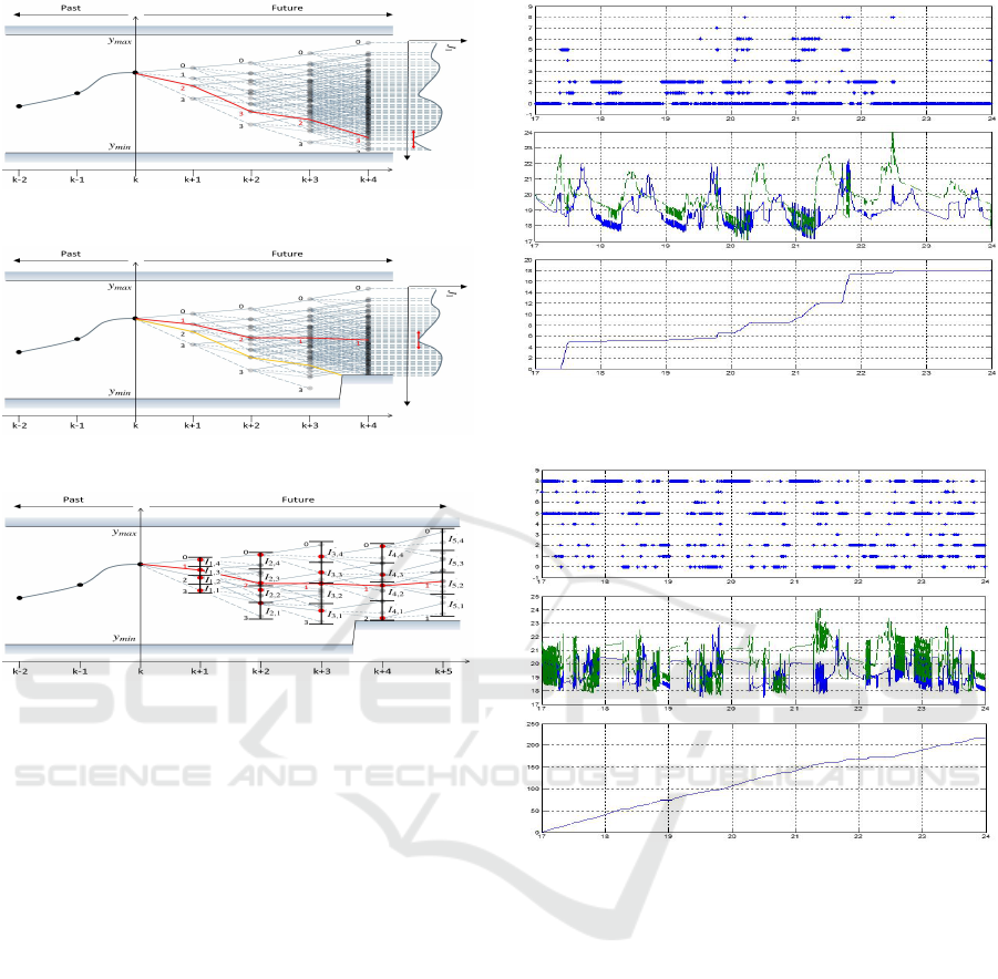
Figure 9: Control scenario predicted from k + 1 until k + 4
for y
min
and y
max
constant.
Figure 10: Control scenario predicted from k +1 until k + 4
for time-dependent y
min
and y
max
.
Figure 11: Control scenario predicted for time-dependent
y
min
and y
max
using an iterative approach.
In this expression, ˆy(k)=y(k) and ˆy
i
j
(k+ j)| ˆy(k+j−1)
represents n predictions of y at k + j from the model
associated with control scenario i
j
and from n parti-
cular predictions of y made the iteration before ( j−1).
At each of the intervals I
j,l
is joined a set of pre-
dictions ˆy
i
α
(k + j). In order to remove the control
scenarios associated to a more important energy cost
than others, it keeps only a unique prediction ˆy(k + j)
per interval I
j,l
. It corresponds to the smallest value
of ˆy
i
α
(k + j). Figure 11 represents the principle of
the proposed iterative approach on the same example
as before with n = 4, N = 5, i
j
∈

0,...,3

= I and
|I| = 4: number of members of I. At every moment of
prediction, the n best predictions ˆy(k + j) (in the sense
of cost function J
1
) are represented in red on the dia-
gram. It can be observed that the scenario of optimal
control i
1
= 1, i
2
= 2, i
3
= 1 and i
4
= 1 is the same
as one obtained by considering all the control scenar-
ios in a comprehensive way. On the other hand, the
computational load is greatly reduced with the itera-
tive algorithm. Indeed, if the number of calculations
to predict ˆy(k + j) is of |I|(nN − n + 1) for this al-
gorithm when dim (y) = 1, it becomes maximum of
(|I|
N+1
− |I|)/(|I| − 1) by exhaustive research.
Figure 12: (a) Control scenarios, (b) temperature of rooms
T
1
,k
(blue) and T
5
,k
(green), (c) kW h energy cost for Q =
0 and N = 30.
Figure 13: (a) Control scenarios, (b) Temperature of rooms
T
1
,k
(blue) and T
5
,k
(green), (c) kW h energy cost for Q =
diag([10
4
0 0 0 10
4
]) and N = 3.
4.3 Simulation tests
Aiming to illustrate the above approach and know-
ing that the main rooms of the platform are
1

and
5
 rooms, the vectors y
min
and y
max
are chosen
such that y
min
=

18 16 16 16 18

and y
max
=

23 25 25 25 23

. Figures 12 - 13 represent the
evolution of temperatures T
1
,k
and T
5
,k
as well as
the different scenarios of the control with their as-
sociated energy cost in kWh over the period 17/05 -
23/05/2016 for different values of N and Q. The in-
puts of the simulator are T
ext,k
(Figure 14), Sol
west
k
and Sol
east
k
(figure 15b) and Occ
k
(figure 15a). By
these different simulations, the effect of the term
∑
N
j=1
||
y
i
j
(k + j) − y
re f
||
2
Q
can be clearly seen on the
optimal order scenario. The more
k
Q
k
is important,
the more actuators with high power energy are so-
Energy Efficiency of a Multizone Office Building: MPC-based Control and Simscape Modelling
233

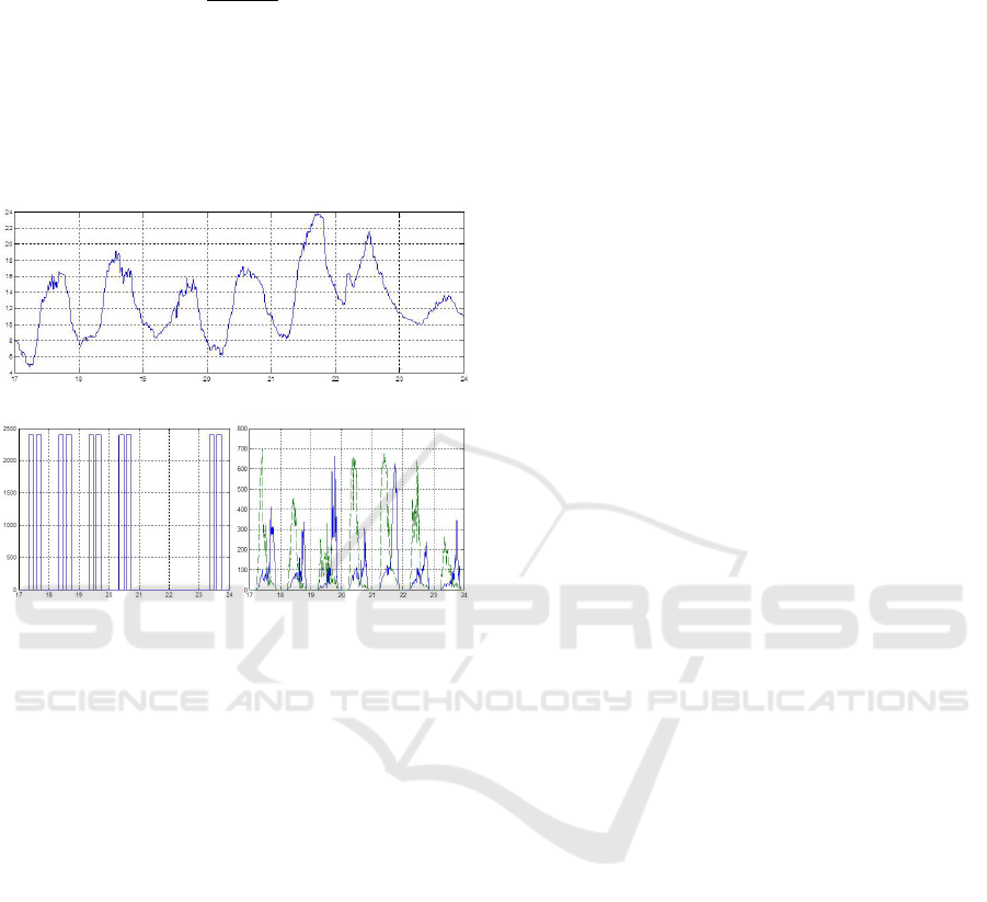
licited (HP in our case) in on-off (hot-cold) control
in order to maintain the temperature of the rooms
1

and
5
 close to y
re f
=
y
min
+y
max
2
= 20.5
◦
C. This type
of scenario is highly energy-consuming (see Figure
13c compared to Figure 12c). Similarly, a low predic-
tion horizon N makes the control more pre-emptive,
resulting in a slight increase in the cost of energy in
kW h. N equal to 30 samples (equivalent to 150 min-
utes) seems to be the best adapted in view of the abil-
ity of cooling/warming of the two HP.
Figure 14: Outside temperature (17/05 - 23/05/2016).
Figure 15: (a) Occ
k
, (b) Solar energy (W ) Sol
west
k
(green)
and Sol
east
k
(blue).
5 CONCLUSION
In this paper, a whole simulator of the thermal be-
haviour of a building platform has been established.
In a relatively high order (72), this simulator inte-
grates the behaviours of the set of the partitions wall
dividers/walls/windows of the platform rooms and all
energy sources (solar radiation, temperature, rooms’
occupancy, ventilation (CMV), heat pumps). Based
on a multi model representation of the building and
on an energy cost function in kWh, a predictive con-
trol has been successfully implemented to ensure the
thermal comfort of the platform rooms with a mini-
mum of energy consumption.
ACKNOWLEDGEMENTS
This work was supported by the 7th Framework Pro-
gramme FP7-NMP-608981 ”Energy IN TIME” and
has financial support from the Contrat de Plan Etat-
R
´
egion (CPER) 2015-2020, project ”Mat
´
eriaux, En-
ergie, Proc
´
ed
´
es”.
REFERENCES
Achterbosch, G. G. J., Jong, P. P. G. D., Krist-Spit, C. E.,
Meulen, S. F. V. D., and Verberne, J. (1985). The de-
velopment of a convenient thermal dynamic building
model. Energy and Buildings, 8:183–196.
Agbi, C. (2014). Scalable and Robust Designs of Model -
Based Control Strategies for Energy - Efficient Build-
ings. Dissertations, Carnegie Mellon University -
http://repository.cmu.edu/dissertations/333.
Antonic, O. (1998). Modelling daily topographic solar radi-
ation without site-specific hourly radiation data. Eco-
logical modelling, 113(1-3):31–40.
ASHRAE (2013). ASHRAE Handbook - Fundamentals (SI
Edition). American Society of Heating, Refrigerating
and Air-Conditioning Engineers, Inc.
Atam, E. and Helsen, L. (2016). Control-oriented thermal
modeling of multizone buildings: Methods and issues:
Intelligent control of a building system. IEEE Control
Systems, 36(3):86–111.
Camacho, E. F. and Bordons, C. (2007). Model predictive
control. Advanced textbooks in control and signal pro-
cessing. Springer-Verlag London.
Goyal, S., Ingley, H. A., and Barooah, P. (2013).
Occupancy-based zone-climate control for energy-
efficient buildings: Complexity vs. performance. Ap-
plied Energy, 106:209–221.
Lapusan, C., Balan, R., Hancu, O., and Plesa, A. (2016).
Development of a multi-room building thermody-
namic model using simscape library. Energy Proce-
dia, 85:320–328.
Le, K., Bourdais, R., and Gueguen, H. (2014). Optimal
control of shading system using hybrid model predic-
tive control. In 2014 European Control Conference
(ECC), pages 134–139, Strasbourg, France.
Lofberg, J. (2004). Yalmip: a toolbox for modeling and
optimization in matlab. In 2004 IEEE International
Symposium on Computer Aided Control Systems De-
sign (CACSD), pages 284–289, Taipei, Taiwan.
Ma, Y., Borrelli, F., Hencey, B., Coffey, B., Bengea, S.,
and Haves, P. (2011). Model predictive control for the
operation of building cooling systems. IEEE Transac-
tions on Control Systems Technology, 20(3):796–803.
Oldewurtel, F., Parisio, A., Jones, C. N., Gyalistras, D., Gw-
erder, M., Stauch, V., Lehmann, B., and Morari, M.
(2012). Use of model predictive control and weather
forecasts for energy efficient building climate control.
Energy and Buildings, 45:15–27.
Privara, S., Siroky, J., Ferkl, L., and Cigler, J. (2011). Model
predictive control of a building heating system: The
first experience. Energy and Buildings, 43(2-3):564–
572.
Scherer, H., Pasamontes, M., Guzman, J., Alvarez, J., Cam-
ponogara, E., and Normey-Rico, J. (2014). Effi-
cient building energy management using distributed
model predictive control. Journal of Process Control,
24(6):740–749.
SMARTGREENS 2017 - 6th International Conference on Smart Cities and Green ICT Systems
234