Detection and Classification of Holes in Point Clouds

Nader H. Aldeeb and Olaf Hellwich

Computer Vision and Remote Sensing, Technische Universität Berlin, Berlin, Germany

nader.h.aldeeb@gmail.com, olaf.hellwich@tu-berlin.de

Keywords: Point Cloud, Hole Detection, Hole Classification, Hole Filling, Surface Reconstruction, Textureless

Surfaces, Segmentation with Graph Cuts.

Abstract: Structure from Motion (SfM) is the most popular technique behind 3D image reconstruction. It is mainly

based on matching features between multiple views of the target object. Therefore, it gives good results only

if the target object has enough texture on its surface. If not, virtual holes are caused in the estimated models.

But, not all holes that appear in the estimated model are virtual, i.e. correspond to a failure of the

reconstruction. There could be a real physical hole in the structure of the target object being reconstructed.

This presents ambiguity when applying a hole-filling algorithm. That is, which hole should be filled and

which must be left as it is. In this paper, we first propose a simple approach for the detection of holes in

point sets. Then we investigate two different measures for automatic classification of these detected holes in

point sets. According to our knowledge, hole-classification has not been addressed beforehand. Experiments

showed that all holes in 3D models are accurately identified and classified.

1 INTRODUCTION

Generating accurate 3D image reconstruction has

found its application in a wide variety of fields, such

as computer aided geometric design, computer

graphics, virtual reality, computer vision, medical

imaging, human computer interaction, computer

animation, and robotics. Because of the availability

of relatively cheap sensors, surface reconstruction

has gained considerable interest (Zaman et al.,

2016). Nowadays, many simple applications that are

based on Structure from Motion (SfM) allow users

to create own high-quality 3D models on their

smart-phones not requiring any experience or

specific knowledge regarding that technique

(Muratov et al., 2016). SfM is based on matching

correspondences between multiple views of the

target object. That matching is based on

correspondence establishing of features such as

corner points (edges with gradients in multiple

directions) from one image to the other. Therefore,

feature detection is highly needed in SfM. One of

the most widely used feature detectors is the Scale-

Invariant Feature Transform (SIFT) (Lindeberg,

2012). Unfortunately, the performance of the SIFT

algorithm over texture-less surfaces is poor, because

no feature point can be detected in such surfaces

(Alismail et al., 2016). Consequently, SfM technique

fails to estimate 3D information in regions having

weak texture information, where no matching points

can be found (Saponaro et al., 2014). That is the

reason why most of the popular 3D reconstruction

techniques give good results only if the target object

has enough texture on its surface. If not, virtual

holes appear in the estimated models. For this kind

of low-textured objects, laser scanners are frequently

used instead of the traditional image based 3D

reconstruction techniques. But, holes may also

appear in the resulting models due to surface

reflectance, occlusions, and accessibility limitations

(Wang et al., 2007).

These days, having a high-quality reconstruction

of objects is an essential demand by many

applications. Therefore, hole-filling or surface

completion has become an important component in

3D image reconstruction process. But, no hole filling

can be applied without the detection of holes in point

clouds. So, hole-detection in point sets is also an

important component in that process. Usually, 3D

image reconstruction methods produce unstructured

point clouds. That is, there is no explicit

connectivity information encoding the surface of the

object. This makes the problem of the detection of

holes on the surface an ill-defined problem (Bendels

et al, 2006).

It is worth mentioning that not all holes

appearing in the estimated model are virtual, i.e. due

to missing reconstructions of featureless surfaces.

Aldeeb N. and Hellwich O.

Detection and Classiﬁcation of Holes in Point Clouds.

DOI: 10.5220/0006296503210330

In Proceedings of the 12th International Joint Conference on Computer Vision, Imaging and Computer Graphics Theory and Applications (VISIGRAPP 2017), pages 321-330

ISBN: 978-989-758-227-1

321

Some of the holes may also represent a real physical

hole, which is part of the structure of the object

being reconstructed. Unfortunately, just looking at

the point cloud, it is almost impossible to

differentiate between these two types of holes (real

and virtual). Particularly, when there is a real

physical hole in the structure of the target object

having uniformly distributed inner-color or inner-

details not appearing in the 2D views, this kind of

regions will appear as regions missing depths in the

estimated model. These are real holes that should be

left as they are during the filling process.

The ambiguity in differentiating between real

and virtual holes is a significant problem, which is

usually faced when running a hole-filling algorithm.

Thus, analysing each of the detected holes and

classifying them to either real or virtual hole is a

very important component in hole-filling process.

Finally, it is now clear that the problem of hole-

filling in point clouds requires two tasks. First,

identifying the holes, and then classifying them. By

classification, the necessity of filling the identified

hole can be determined. Unfortunately, both tasks

are nontrivial. But in this paper, we propose a simple

approach which will contribute to the accurate

detection and classification of holes in point clouds,

and consequently support systems for surface

reconstruction and hole filling.

The rest of this paper is organized as follows:

section 2 presents a brief background and lists the

related work. Section 3 discusses the proposed

approach. Experimental results and discussion can

be found in section 4. Finally, section 5 concludes

with a conclusion, perspectives, and future work.

2 BACKGROUND AND RELATED

WORK

Structure from Motion (SfM) techniques have

attracted researchers since the work of (Tomasi and

Kanade, 1992). SfM algorithm involves finding

correspondences between different input images for

the object being reconstructed, and then estimates a

3D model and a set of camera parameters.

Therefore, reconstructing regions having low

textures is challenging for most of SfM-based

approaches.

As mentioned before, the need for accurate 3D

models makes hole-filling a very important problem.

For a successful hole-filling, accurate detection and

classification of holes in point clouds are needed.

According to our knowledge, and after an intensive

review of the literature, not much work has been

published about detecting holes in point clouds.

Nevertheless, some methods employed either special

equipment or triangular meshes, sometimes

associated with some input entered manually by

users for hole-identification. For example, in (Noble

et al., 1998), the internal geometry feature of 3D

objects is measured by employing an X-ray

inspection method; thereby they were able to

position the drilled holes on the object's surface. In

(Kong et al., 2010), a hole-boundary identification

algorithm for 3D closed triangle mesh is presented.

In this method, the user has to interactively select

the region of interest by mouse dragging. From our

point of view, this method has one more drawback

besides the need for manual inputs. Dependence on

meshes instead of point clouds will not guarantee the

detection of all holes, because some meshing

algorithms may fill the regions of missing depth.

Consequently, this prevents distinguishing real from

virtual holes.

The authors of (Wang et al., 2012) proposed a

method which aims to find solid holes inside 3D

models. This method is also based on triangular

mesh models. By grouping interconnected coplanar

triangles, they extract the contour of the model using

the boundaries of the adjacent planes. Then, based

on the extracted contour, they form several disjoint

clusters of model vertices. Finally, by analysing the

relationship between the clusters and planes, holes

are identified. But, this method only finds solid

holes inside models, and does not detect regions of

missing depths.

The main goal of (Wang et al., 2007) is filling

holes in locally smooth surfaces. But, as a pre-

processing step, holes are found based on the

triangular mesh of the input point cloud. In this

method, holes are identified automatically by

tracking boundary edges. If an edge belongs only to

a single triangle, then it is a boundary edge,

otherwise it is a shared edge, which shares more

than one triangle. But, employing this strategy in

finding holes will detect all holes including the real

holes those need not be filled. Therefore, in this

work, user input is required as an assistance. So,

again, manual user inputs are needed in this work.

An automatic hole-detection approach has been

presented in (Bendels et al., 2006). Properties of

point sets have been investigated to derive several

criteria which are then combined into an integrated

boundary probability for each point. This method

seems to be robust, but we have noticed that it has

some drawbacks. First, in their combination of

probability criteria, they used some weights, which

VISAPP 2017 - International Conference on Computer Vision Theory and Applications

322

have to be set by the user according to visual

inspection. Second, they have a set of predefined

parameters, which limits the scalability of the

approach. For example, a predefined diameter is set

for the hole to be detected.

Some other approaches address a closely related

problem. For example, (Dey and Giesen, 2003)

present an approach for the detection of under-

sampled regions. The detection is guided using a

sampling requirement, which has been defined to

ensure a correct reconstruction of surfaces. For

example, for correct reconstruction, every point on

the surface should have at least one sample point

within a ball with a predefined size. But, according

to this definition, their method will not succeed in

detecting holes in planar regions, where this

requirement is mostly fulfilled by a little number of

samples.

3 THE PROPOSED ALGORITHM

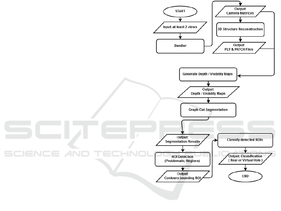
Fig. 1 shows the flowchart of the proposed

algorithm. In the following subsections, each of the

main processes will be discussed in brief using

demonstration examples.

3.1 Input a Number of Views

The first step in the proposed algorithm requires a

number of input images. Because the technique

proposed in this paper uses stereo correspondences,

two calibrated images from different viewpoints for

the object being reconstructed are needed at least.

3.2 Bundle Adjustment

Bundle Adjustment is the process of jointly refining

a set of initial camera and structure parameter

estimates for finding the set of parameters, which

most accurately predict the locations of the observed

points in the set of available images (Alismail et al.,

2016). Assuming we have n 3D points that are seen

in m views, and the projection of the i

point into

view j is denoted by X

, and let v

be a binary

number equals 1 if the point i is visible in view j and

0 otherwise. Also, let a

denote the vector carrying

the parameters of camera j and b

is the vector

carrying the coordinates of the 3D point i. Then by

minimizing the following energy function, we get

the optimal projection matrix for each camera.







































(1)

where, Q(a

) denotes the predicted projection of

point i onto view j and d(x,y) denotes the Euclidean

distance between the image points x and y. In our

research, we used Bundler (Snavely et al., 2008;

Snavely et al., 2006) for getting the camera matrices.

Figure 1: Flowchart of the proposed approach, detection

and classification of holes in point clouds.

3.3 Reconstruction of the 3D Structure

Patch-based Multi-View Stereo (PMVS) software

(Furukawa and Ponce, 2010) has been employed to

reconstruct the 3D structure of objects visible in

images. According to our proposed approach, we

need to know the views in which the generated 3D

points are visible. One of the outputs generated by

PMVS is the PATCH file, which contains full

reconstruction information. That includes the

number of reconstructed 3D points, the 3D location,

the normal, and photometric consistency score for

each point. Also, it states the number of images in

which the point is visible as well as the actual image

indexes. That is the main reason for using PMVS in

our implementation.

Detection and Classiﬁcation of Holes in Point Clouds

323

3.4 Generating Depth and Visibility

Maps

The goal of this research is to analyse the 3D

structure of objects appearing in images through

investigating the combination of the 3D structure

together with the features and details provided by

the images. Therefore, the goal of this process is to

relate the 3D information, which we got in the

previous process, with the 2D views (images).

In point clouds, each point can be denoted using

a homogeneous 3D coordinate as (x y z 1). Similarly,

the homogeneous 2D coordinate of its projection

into images can be denoted as (u v 1). From the

patch file, we know the view in which each of the

3D points is visible. Then, using the corresponding

camera matrix, P, we can relate each 3D-coordinate

to its 2D-coordinate by following (2), where d is the

depth of that point.











 









(2)

We can thus generate depth-maps for our object

based on all its views (images). Because images are

10 times down sampled, the value of each pixel in

that map is the average of the depth values of the

projected 3D points into that pixel location. If for a

given pixel no depth information is given, it is

assigned a depth equals



 times the maximum

depth in the map (very far). Thereby, we guarantee

that the generated value is larger than the maximum

depth in the map. Here, it is worth mentioning that

values other than



 can also be used. But the used

value has a direct effect in segmentation, as it will

become clear in section 3.5.2.

Also, exploiting the visibility information from

the PMVS's PATCH file, we can generate visibility-

maps, where each pixel is assigned a number which

equals the total number of 3D points which are

projected to that pixel location. This happens

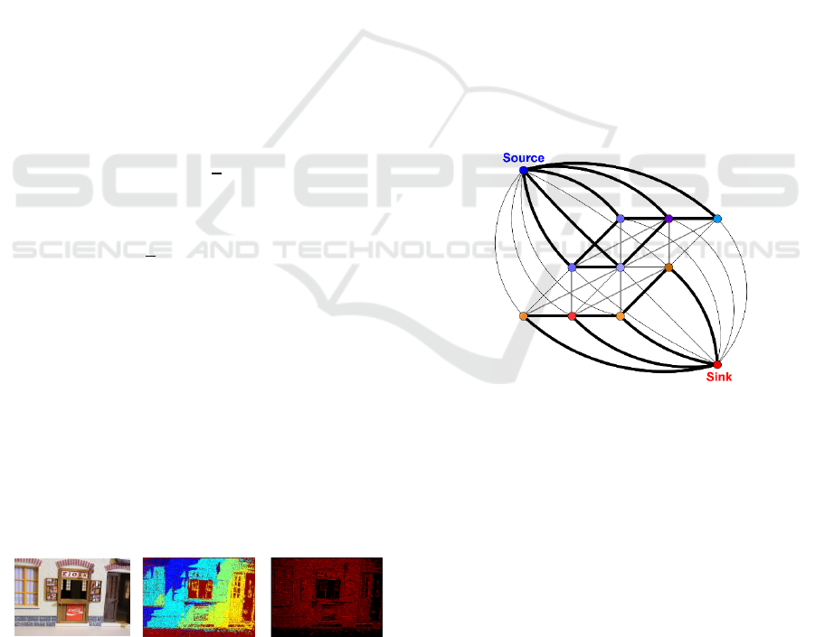
because of the down sampling of images. Fig. 2

shows both maps for one view of the house model as

an example (see section 4 for more details about the

dataset). In the visibility-map, for demonstration, a

pixel is marked red if it has depth information in the

generated 3D structure and marked black otherwise.

(a)

(b)

(c)

Figure 2: Example depicting (a) original image, (b) depth-

map and (c) visibility-map.

Afterwards, we will use either of these maps to

identify the problematic regions, which have no

depth information, out of each image employing

graph cuts.

3.5 Segmentation using Graph Cuts

To take advantage of the competent solutions of

graph-based approaches for segmentation problems,

we built an s-t-graph (Boykov and Funka-Lea,

2006). The number of nodes in the graph equals to

the number of pixels in the input map. Two more

additional nodes, the source and the sink, represent

the segmentation labels. Each node in the graph is

connected to its 8-neighborhood nodes based on the

neighbourhood information of pixels. In addition,

each node is joined to the source and the sink using

two weights, which represents the likelihood of the

corresponding pixel to either of the segmentations

labels. Fig. 3 shows a sketch of the graph. For

accurate segmentation results, weights form

different types of regions must assure a large

difference. For reasons of comparison, weights are

selected based on the depth-maps one time and on

the visibility-maps at the other time.

Figure 3: Sketch of the graph and connectivity

(w3.impa.br/~faprada).

3.5.1 Supporting Graph Cut Segmentation

For supporting our graph-based segmentation,

before we set the weights for the graph, we estimate

another kind of segmentation, which gives an

indirect indication about the nature of pixels. That is,

whether they have depth information or not. Since

SfM techniques perform poorly in regions having

weak or no textures, we first detect these regions in

original images, then each pixel is classified to

belong either to a textured or texture-less region.

Finally, weights on graph edges are affected by

those classification results.

VISAPP 2017 - International Conference on Computer Vision Theory and Applications

324

According to (Scharstein and Szeliski, 2002),

texture-less regions are defined as regions where the

average of the squared horizontal gradient over a

predefined window is below some given threshold.

Using (3), we get the squared horizontal intensity

gradient for two neighbouring pixels. It is calculated

over the three color-channels, c, and then averaged.

If we repeat this for all pixels in image, we get the

Gradient Image GI, where i and j are the image’s

row and column indices respectively.





  























 



  









(3)

If for a given region, which is covered by a window

of a predefined size S×S, the average of the squared

gradient is less than some predefined threshold T,

then this region is assumed as a texture-less region.

The average squared gradient over a predefined

window can be calculated as:

 







  





    





(4)

Image indices i and j are set such that the window

remains inside the image boundaries each time the

Avg is calculated. Pixels falling in weak or texture-

less regions are assigned the value β = 1, (white

color). All other pixels are assigned the value β = 0,

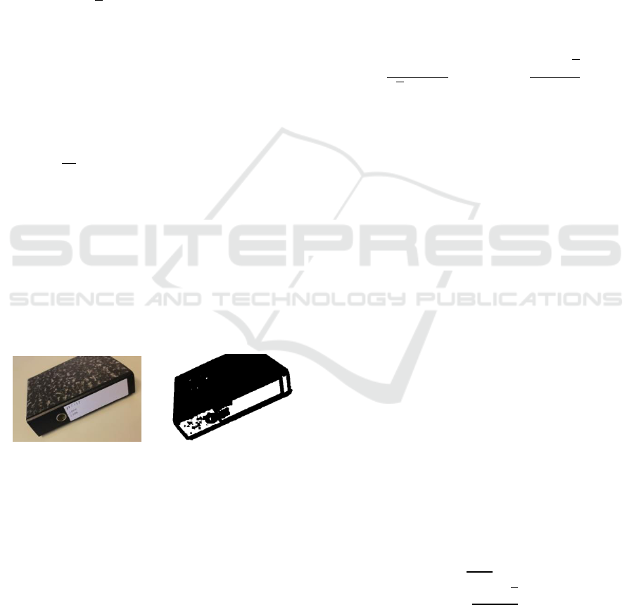
(black color). Fig. 4 shows the classification results

for one view of the Folder model (see section 4 for

more details about the dataset). We used the

parameters S=9 and T=3.

(a)

(b)

Figure 4: Example showing (a) original image, (b)

“textured”, ‘texture-less” classification results.

3.5.2 Segmentation based on Depth-Maps

Based on depth-maps, the weights of the graph are

given in a way such that the min-cut / max-flow

goes through regions where no depth information is

available. If the maximum depth for a given depth-

map, D, is D

max

, and the depth for a given point, p, is

D(p), the term weight, W

, is estimated using (5).

Where, β

is the supporting parameter, which is the

classification of the pixel corresponds to point p (see

section 3.5.1). And α is a tuning parameter, used to

suppress the effect of the supporting term. This kind

of suppression is very important, because the

presence of a pixel in a textured region, β

= 0, does

not guarantee that we have a corresponding depth

information. This usually happens if the pixel is not

visible in other views. Therefore, we set α to 10, this

has the effect of a little decrease in point weight. It is

worth mentioning that if a pixel falls in a texture-less

region, β

= 1, then the supporting term becomes

zero. So, the maximum possible point weight is

guaranteed. This makes sense, as there will be no

corresponding depth information for that pixel.

Basically, W

is the probability that point p belongs

to a problematic region.

















  



   



 























(5)

In addition, each edge, E

, which connects any two

points, p and q, is assigned two weights, W

and

, as seen in (6) and (7) respectively.





 



(6)











   



 



  



 

(7)

Fig. 5 (b) shows the result of segmenting a depth-

map, which has been shown in Fig. 2 (b). White

color is used to refer to pixels having no depth

information.

3.5.3 Segmentation based on Visibility-maps

As in section 3.5.2, the weights of the graph are

given such that the min-cut / max-flow goes through

the problematic regions, but now based on the

visibility-maps. Based on our definition of a

visibility-map, V, problematic regions are the

regions composed of pixels that have the least

number of projections. Therefore, these points are

given highest weight in the graph. For some given

point, p, which has the total number of projections

V(p), the term weight, W

, is estimated as in (8).

Note that here we also use a supporting term, which

is exactly same as the term used in section 3.5.2.





   





    

















(8)

Also, each edge, E

, is assigned two weights, W

and W

, which are calculated as in section 3.5.2 but

now point weights are estimated using (8). Fig. 5 (c)

Detection and Classiﬁcation of Holes in Point Clouds

325

shows the result of segmenting a visibility-map,

which has been shown in Fig. 2 (c). White color is

used to refer to pixels having no depth information.

(a)

(b)

(c)

Figure 5: Segmentation results for both maps shown in Fig

2. Part (a) is the original point cloud, (b) depth-map

segmentation, and (c) visibility-map segmentation.

At first glance, segmentation results look in

somehow the same and this might also be supported

theoretically. Because if we have a 3D point, this

means for sure that it is visible in at least two of the

views, so depth means visible. But, for the detection

of the problematic regions, we prefer depending on

depth-map-based segmentations for the following

reason: Taking the exact depth value of each point

for weighting the graph is more efficient and robust

than taking the cue that the point is visible in the

view. Because, the noisy 3D points will be noted as

visible in views, and will contribute in weight

estimations with the same amount as the non-noisy

points. But based on depth-maps, noisy points,

which have been assigned erroneous depths, will

contribute with their depths, which will be different

from the other non-noisy points depths.

3.6 Regions of Interest (ROI) Detection

In this process, we need not only delineate the

problematic regions, but also, we need a direct

access to the points inside those regions for further

processing. Therefore, contours will be the most

appropriate tool fulfilling our demand. We also need

the detected contours to be closed. I.e., the

boundaries or edges of the problematic regions need

to be connected. In the segmentation results, which

we already saw in Fig. 5, the problematic regions,

those having no depth information, are tightly

delineated or connected. So the detection of such

regions using closed contours is quite easy. But,

after many observations, we have noticed that this

might not be the case all the time. This presents

challenges in the detection process. Therefore, as an

attempt to connect the non-connected edges, we

decided to first detect the edges of the object being

reconstructed using the original images, and then

combine the detected edges with the segmentation

results. Fig. 6 shows an example, where this

combination helps in detecting closed contours

surrounding ROI. As shown in (d), it is clear that the

contours are not tightly delineating the problematic

regions. But after the inclusion of the object's

detected edges to the segmentation edges, as shown

in (e), the detected contours are now delineating the

problematic regions in a helpful manner, as seen in

part (f).

(a)

(b)

(c)

(d)

(e)

(f)

Figure 6: Example depicting the benefit of combining both

depth and real edges in the process of ROI detection. (a)

Original Image. (b) depth-map segmentation. (c) Detected

edges based on (b). (d) Detection of the ROI based on (c).

(e) Combining both the original object edges with the

depth based edges shown in (c). (f) Detection of the ROI

based on (e).

3.7 Classification of the Detected

Problematic Regions

After the detection of the problematic regions in

images, simple approaches are investigated to check

their performance in the classification of the

detected regions.

First, we conduct a statistical measure on the

pixels in each problematic region to be classified.

This measure assumes that the behaviour of each

ROI among the views should tell about the nature of

it. This assumption has been inspired from the fact

that the human does the same whenever holes are to

be recognized by looking for details inside the hole,

like the shadow. For the sake of robustness, the

calculations are done using Hue-Saturation-Value

(HSV) color-space. Because, HSV separates the

image intensity from the color information (Haluška

et al., 2015). For the classification of a given

detected problematic region P, which appears in n

views, we first find the mean set, 













, where 



is the average intensity

inside the region P in view i. Then we find the

variance and standard deviation of the set M as 













 







, and  







respectively,

where µ is the mean of the set M. Finally, we make a

list of pixels appearing inside the problematic region

P in all the views and check each pixel p whether it

satisfies the condition         or

VISAPP 2017 - International Conference on Computer Vision Theory and Applications

326

not. If the percentage of pixels satisfying that

condition exceeds a given threshold, T (see section

4), then P is assumed as a virtual hole, otherwise it is

assumed as a real hole.

Second, we experiment a depth measure, which

re-projects the problematic region to be classified

into the 3D space and simply differentiates the

average depth of the 3D points on the contour

delineating the region from that inside the same

region. If the region corresponds to a real physical

hole, then it is supposed to have a significant depth

difference. Otherwise, if the region corresponds to a

virtual hole, the difference is supposed to be

negligible. A depth threshold, T

, is used for that

reason (see section 4).

4 EXPERIMENTAL RESULTS

As mentioned before, hole-classification has not

been addressed beforehand. Therefore, no

comparisons to other works will be given in this

section. However, many experiments have been

conducted to investigate the performance of the

proposed approach in terms of accuracy in detecting

and classifying holes. The material used in this part

includes a dataset of 55 models for different indoor

objects and scenes, each of which is reconstructed

using VisualSFM (Wu, 2011) based on a set of

images (5184 x 3456) taken from different

viewpoints. For performance issues, after estimating

the 3D models, all images are 10 times down

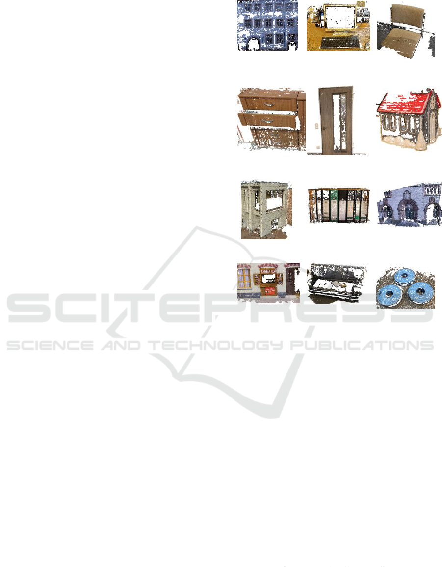
sampled. Fig. 7 shows a sample set of the models

used in this paper.

The reconstructed models contain many

problematic regions, with size ranges from 600 to

150,000 pixels. The size of a problematic region P is

the least number of pixels appear in P when

projected to each of the down-sampled views. As a

ground truth, we make a record of randomly selected

set of problematic regions, each of which is assigned

to either real or virtual hole. 40% of the selected set

are for real holes and 60% are for virtual holes.

Training our statistical and depth classifiers is to

estimate the values of thresholds, T and T

, by which

problematic regions can be classified. For that

reason, 20 models are selected randomly for

training. Many observations have been applied for

different values of these thresholds. The accuracy

corresponds to each observation has been recorded.

The highest average classification accuracy was

obtained when setting T = 30 % and T

= 0.01

(normalized).

(a) Castle-P19

(Strecha, 2008)

(b) Screen

(d) Drawer.

(e) Door.

(f) Tiny House.

(g) Hall.

(h) Shelf.

(i) Herz-Jesu-P8

(Strecha, 2008).

(j) House.

(k) Sofa.

(l) Wheels.

Figure 7: Some of the models used in evaluating the

proposed approach.

4.1 Evaluating the Detection of the

Problematic Regions

Figure 8 shows an example of problematic regions

detection. As mentioned before, contours are used to

delineate the problematic regions. Therefore, to

quantitatively assess the detection accuracy, we

measured the similarity between the detected

contour and the ideal contour, which is set manually.

This has been done for a set of the test models. The

similarity between contours is measured using the

Pratt’s Figure of Merit (PFOM) (Abdou and Pratt,

1979) defined in (9). This measure basically depends

on estimating the distance between point pairs of the

two contours.

 

















  











(9)

Detection and Classiﬁcation of Holes in Point Clouds

327

Where, I

and I

are the numbers of edge points in

the ideal, ground truth, and the detected contour

respectively. d

is the distance between the i

pixel

in the detected contour and the nearest pixel in the

ideal contour. Finally, α is an experimental constant

which was set to 1/9 according to (Abdou and Pratt,

1979). The value of R ranges between 0 and 1. The

larger the value of R, the more accurate the detected

contour is. The average value of R we got in this

experiment is 0.89. This value means that

approximately 90% of the ROI is detected. This is

sufficient for the next processing steps to achieve the

goal of this research. This is because 90% of the

region’s area will definitely contain most of the

details, in which we are interested for the next

processing step.

(a)

(b)

(c)

(d)

Figure 8: Demonstrating the detection of the problematic

regions. (a) Toy Model, reconstructed using Visual-SFM

(10 images). (b) detected problematic region in one of the

images used in (a). (c) House Model, reconstructed using

Visual-SFM (10 images). (d) Two detected problematic

regions in one of the images used in (c).

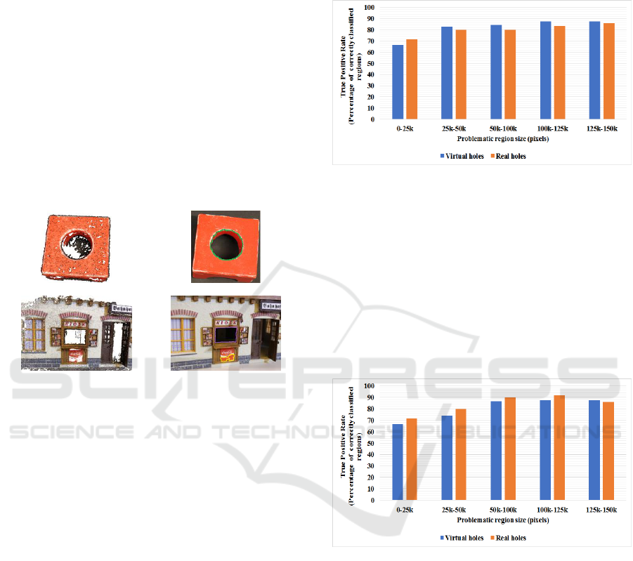
4.2 Evaluating the Classification of the

Problematic Regions

To evaluate the accuracy of the proposed

classification approaches mentioned in section 3.7,

we compare the outcome of the classification

experiments with the ground truth classification. The

average accuracies for classifying virtual and real

holes using the proposed statistical classifier can be

seen in Fig. 9. Problematic regions are categorized

into 6 categories based on their sizes.

The average true positive rates for classifying

virtual and real holes are 81.74% and 80.09%

respectively. As seen in Fig. 8, the smaller the

problematic region is, the lower the true positive rate

we get. Many small virtual holes were classified as

real holes. The reason behind this is the effect of the

change in lighting conditions on those regions from

one view to the other. This effect usually biases our

classifier. Also, many small real holes were

classified as virtual holes. Because the details behind

these holes are not clearly visible.

Figure 9: True positive rates for the statistical classifier.

Figure 10 shows the average accuracies for

classifying virtual and real holes using the proposed

depth classifier. The average true positive rates for

classifying virtual and real holes are 80.44% and

83.76% respectively. In fact, for the latest measure,

the models, in which problematic regions were false

positive or false negative, are either noisy models or

having regions, in which it is very difficult to

calculate the measure because of having no depth

information inside it.

Figure 10: True positive rates for the depth classifier.

4.3 Evaluating the Efficiency of the

Proposed Approach

The results listed in this section were taken using a

personal computer running Windows 7 64-bit

operating system with Intel Core i7 3.6 GHz

processor and 16 GB Memory installed. The

approach has been implemented using C++.

The efficiency of the proposed approach is

highly dependent on the starting point from which

the processing will start, see Fig. 1. The point from

which we start usually depends on which type of

data do we have. If we only have the images of the

VISAPP 2017 - International Conference on Computer Vision Theory and Applications

328

object and still have no 3D reconstruction of it, then

the time consumed by the proposed approach will

include the time for the bundler and 3D

reconstruction pipeline. Unfortunately, these two

components usually take long time, depending on

the size and number of input images (approximately

3 minutes to process 8 images each of which has

size 5184×3456). Nonetheless, the rest of

components in the proposed approach are very

efficient. Fig. 11 shows the average time required

for generating and segmenting depth-maps given

different numbers of input images. It is worth

mentioning that, as the number of the input images

increases, the classifications of the problematic

regions will become more stable. But, as seen in the

figure, the larger the number of views results in

longer processing times. Therefore, a kind of trade-

off is required. In practice a number between 4 and 8

images has proved to be sufficient for achieving the

goal in less than one second. Nevertheless, despite

of having a quite large number of input images, the

required time still less than 1 second for generating

the maps and less than 2.5 seconds for segmenting

them.

Figure 11: Average time required to generate and segment

depth-maps, corresponding to a given number of views.

Finally, to estimate performance of the time

required for the detection and classification of the

problematic regions, we conducted an experiment

using a set of models containing several problematic

regions with different sizes. The average

problematic region detection time we got is 0.0026

second and the average classification times we got

using the statistical and depth classifiers are 0.042

and 0.80 second respectively.

5 CONCLUSION AND FUTURE

WORK

A simple approach for the detection and

classification of holes in point sets is proposed. In

this research, it has been proved that depth-map is a

robust and efficient resource for the detection of

problematic regions in point-clouds. We also proved

that simple statistical measures can be used for the

automatic classification of the detected problematic

regions in point sets. The results of the experiments

we got are quite promising. Holes are accurately

identified and classified. Nevertheless, there are still

some problems that need to be addressed in future.

For example, robustness to lighting variations on

surfaces, as well as to noise in point clouds. Also,

our future work will concentrate in filling holes,

which are classified as virtual holes.

ACKNOWLEDGMENTS

The authors would like to thank the German

Academic Exchange Service (DAAD) for providing

financial support for research studies. We are

grateful to our colleagues who provided insight and

expertise that greatly assisted this research work.

REFERENCES

Abdou, I. E. and Pratt, W. K., 1979. Quantitative design

and evaluation of enhancement/thresholding edge

detectors. Proceedings of the IEEE, 67(5), pp.753-763.

Alismail, H., Browning, B. and Lucey, S., 2016. Direct

Visual Odometry using Bit-Planes. arXiv preprint

arXiv:1604.00990.

Alismail, H., Browning, B. and Lucey, S., 2016.

Photometric Bundle Adjustment for Vision-Based

SLAM. arXiv preprint arXiv:1608.02026.

Bendels, G. H., Schnabel, R. and Klein, R., 2006.

Detecting holes in point set surfaces.

Boykov, Y. and Funka-Lea, G., 2006. Graph cuts and

efficient ND image segmentation. International

journal of computer vision, 70(2), pp.109-131.

Dey, T. K. and Giesen, J., 2003. Detecting undersampling

in surface reconstruction. In Discrete and

Computational Geometry (pp. 329-345).

Furukawa, Y. and Ponce, J., 2010. Accurate, dense, and

robust multiview stereopsis. IEEE transactions on

pattern analysis and machine intelligence, 32(8),

pp.1362-1376.

Detection and Classiﬁcation of Holes in Point Clouds

329

Haluška, J., 2015. On fields inspired with the polar HSV-

RGB theory of Colour. arXiv preprint

arXiv:1512.01440.

Kong, L. X., Yao, Y. and Hu, Q. X., 2010. Hole boundary

identification algorithm for 3D closed triangle mesh.

Computer Engineering, 36, pp.177-180.

Lindeberg, T., 2012. Scale invariant feature transform.

Scholarpedia, 7(5), p.10491.

Muratov, O., Slynko, Y., Chernov, V., Lyubimtseva, M.,

Shamsuarov, A. and Bucha, V., 2016. 3DCapture: 3D

Reconstruction for a Smartphone. In Proceedings of

the IEEE Conference on Computer Vision and Pattern

Recognition Workshops (pp. 75-82).

Noble, J. A., Gupta, R., Mundy, J., Schmitz, A. and

Hartley, R.I., 1998. High precision X-ray stereo for

automated 3D CAD-based inspection. IEEE

Transactions on Robotics and automation, 14(2),

pp.292-302.

Saponaro, P., Sorensen, S., Rhein, S., Mahoney, A.R. and

Kambhamettu, C., 2014, October. Reconstruction of

textureless regions using structure from motion and

image-based interpolation. In 2014 IEEE International

Conference on Image Processing (ICIP) (pp. 1847-

1851). IEEE.

Scharstein, D. and Szeliski, R., 2002. A taxonomy and

evaluation of dense two-frame stereo correspondence

algorithms. International journal of computer vision,

47(1-3), pp.7-42.

Snavely, N., Seitz, S. and Szeliski, R., 2006. Photo

Tourism: Exploring Image Collections in 3D. ACM

Transactions on Graphics.

Snavely, N., Seitz, S. M. and Szeliski, R., 2008. Modeling

the world from internet photo collections.

International Journal of Computer Vision, 80(2),

pp.189-210.

Strecha, C., von Hansen, W., Van Gool, L., Fua, P. and

Thoennessen, U., 2008, June. On benchmarking

camera calibration and multi-view stereo for high

resolution imagery. In Computer Vision and Pattern

Recognition, 2008. CVPR 2008, pp. 1-8.

Tomasi, C. and Kanade, T., 1992. Shape and motion from

image streams under orthography: a factorization

method. International Journal of Computer Vision,

9(2), pp.137-154.

Wang, J. and Oliveira, M. M., 2007. Filling holes on

locally smooth surfaces reconstructed from point

clouds. Image and Vision Computing, 25(1), pp.103-

113.

Wang, Y., Liu, R., Li, F., Endo, S., Baba, T. and Uehara,

Y., 2012, August. An effective hole detection method

for 3D models. In Signal Processing Conference

(EUSIPCO), 2012 Proceedings of the 20th European

(pp. 1940-1944). IEEE.

Wu, C., 2011. VisualSFM: A visual structure from motion

system.

Zaman, F., Wong, Y. P. and Ng, B. Y., 2016. Density-

based Denoising of Point Cloud. arXiv preprint

arXiv:1602.05312.

VISAPP 2017 - International Conference on Computer Vision Theory and Applications

330