Cost Optimization on Public Cloud Provider for Big Geospatial Data:

A Case Study using Open Street Map

Joao Bachiega Junior, Marco Antonio Sousa Reis, Aleteia P. F. de Araujo and Maristela Holanda

Department of Computer Science, University of Brasilia, Brasília/DF, Brazil

Keywords: Big Geospatial Data, SpatialHadoop, Geospatial Cloud.

Abstract: Big geospatial data is the emerging paradigm for the enormous amount of information

made available by the development and widespread use of Geographical Information System

(GIS) software. However, this new paradigm presents challenges in data management, which

requires tools for large-scale processing, due to the great volumes of data. Spatial Cloud Computing offers

facilities to overcome the challenges of a big data environment, providing significant computer power and

storage. SpatialHadoop, a fully-fledged MapReduce framework with native support for spatial data, serves as

one such tool for large-scale processing. However, in cloud environments, the high cost of processing and

system storage in the providers is a central challenge. To address this challenge, this paper presents a cost-

efficient method for processing geospatial data in public cloud providers. The data validation software used

was Open Street Map (OSM). Test results show that it can optimize the use of computational resources by up

to 263% for available SpatialHadoop datasets.

1 INTRODUCTION

Cloud computation is a model that

facilitates transparent, and on-demand, access to a set

of computational resources (for example, networks,

servers, warehousing, applications and services),

which can be acquired quickly, and released

with very little managing effort, or interaction with

the service provider. Kramer and Senner (2015)

affirm that the cloud offers virtually unlimited

resources in terms of processing power and

memory. Subsequently, the amount of computational

resources required by this vast volume of

information, aka big data, grows in an asymptotic

way. Therefore, each computational resource

wasted potentially represents wasted financial

resources – making processing in cloud environments

costly –, since public cloud providers, like Amazon

AWS, Microsoft Azure, Google Cloud and others,

charge users on a pay-per-use basis.

Big data has some specific characteristics that

distinguish it from other datasets (Sagiroglu and

Sinanc, 2013). These characteristics, known as the

7Vs, are (Pramila, 2015): i) Variety – referring to the

different types of data, with more than 80% of them

in an unstructured form; ii) Volume – the tremendous

amount of data generated each second; iii) Velocity –

the speed at which new data is being produced; iv)

Veracity – how trustworthy the data is; v) Value –the

importance of the data to the business; vi) Variability

- data with constantly changing meaning and vii)

Visualization – data presented to users in readable and

accessible way.

Consequently, some methods were developed to

process big data (Sagiroglu and Sinanc, 2013).

Among them, Apache Hadoop stands out. It is a

programming framework for distributed computing

using the divide and conquer (or Map and Reduce)

method to break down complex big data problems

into small units of work and process them in parallel.

The rise of big geospatial data creates the need for

an environment with ample computational resources

in order to process this amount of geographical

information. Some applications were developed

specifically for this big geospatial data using Hadoop

concepts (Eldawy and Mokbel, 2015): i) “GIS Tools

on Hadoop”, which works with the ArcGIS product;

ii) Parallel-Secondo as a parallel spatial DBMS that

uses Hadoop as a distributed task scheduler; iii) MD-

HBase extends HBase, a non-relational database for

Hadoop, to support multidimensional indexes; iv)

Hadoop-GIS extends Hive, a data warehouse

infrastructure built on top of Hadoop with a uniform

Junior, J., Reis, M., Araujo, A. and Holanda, M.

Cost Optimization on Public Cloud Provider for Big Geospatial Data.

DOI: 10.5220/0006237800820090

In Proceedings of the 7th International Conference on Cloud Computing and Services Science (CLOSER 2017), pages 54-62

ISBN: 978-989-758-243-1

grid index for range queries and self-join. Finally,

Eldawy and Mokbel (2015) presented SpatialHadoop,

a fully-fledged MapReduce framework, with native

support for spatial data with better performance than

all the other applications listed.

One challenge in a cloud environment is to know

the cost of processing big data in public cloud

providers. According to Zhang et al (2010),

cloud computing has impact where large companies,

such as Google, Amazon and Microsoft, strive to

provide cost-efficient cloud platforms. In this way,

the cost to execute the applications using these public

providers is fundamental information for executing

applications in a cloud. In this context, this article

presents a method for cost-efficient processing in

public cloud providers for big geospatial data using

SpatialHadoop. For this, an Open Street Map (OSM)

dataset is used with the goal of optimizing the use of

computational resources to reduce costs.

The remainder of the article is divided into 5

sections. Section 2 covers concepts of Spatial Cloud

Computing, SpatialHadoop and some related works.

Section 3 presents the method to determine the

number of data nodes in a cluster, based on dataset

size. The case study is presented in Section 4, with

information about architecture, datasets, tests and

results. Finally, Section 5 contains the conclusion and

some suggestions for future work.

2 THEORICAL REFERENCE

In this section, concepts about cloud computing will

be presented, highlighting the characteristics for an

environment to process big geospatial data and, also,

about SpatialHadoop, and related works.

2.1 Spatial Cloud Computing

Although computing hardware technologies,

including a central processing unit (CPU), network,

storage, RAM, and graphics processing unit (GPU),

have advanced greatly in past decades, many

computing requirements for addressing scientific and

application challenges, such as those for big

geospatial data processing, exceed existing

computing capabilities (Yang et al., 2011).

These challenges require a computing

infrastructure that can: i) support data discovery,

access, use and processing well, relieving scientists

and engineers of IT tasks so they can focus on

scientific discoveries; ii) provide real-time IT

resources to enable real-time applications, such as

emergency response; iii) deal with access spikes; and

iv) provide extremely reliable and scalable service for

massive numbers of concurrent users to advance

public knowledge (Eldawy et al., 2015).

Cloud computing offers facilities to overcome the

challenges of a big data environment, providing

substantial computer power and vast storage. In the

most common definition of cloud computing, NIST

(2011) indicates five essential characteristics,

namely, on demand self-service, broad network

access, resource pooling, rapid elasticity, and

measured service.

However, other characteristics are relevant to

defining spatial cloud computing environments.

Akdogan et al. (2014) proposed a cost-efficient

partitioning of spatial data in clouds. This partitioning

method considers location-based services and

optimizes the storage of spatial-temporal data to be

able to turn-off idle servers and reduce costs.

Yang et al. (2011) defines Spatial Cloud

Computing as the cloud computing paradigm that is

driven by geospatial sciences, and optimized by

spatiotemporal principles for enabling geospatial

science discoveries and cloud computing within a

distributed computing environment. This is expected

to supply the computational needs for geospatial data

intensity, computing intensity, concurrent access

intensity and spatiotemporal intensity.

According to NIST (2011), there are four

deployment models for clouds, namely private,

community, public and hybrid. Specifically, to public

clouds, the authors define how the cloud

infrastructure is provisioned for open use by the

general public. In this model of cloud deployment,

services are charged for using a pay-per-use method

at some level of abstraction appropriate to the type of

service (e.g. storage, processing or bandwidth). When

working with big geospatial data, the volume of data

and the power of processing are always high and,

subsequently, expensive.

According to the “Gartner Magic Quadrant for

Cloud Infrastructure as a Service”, Amazon AWS is

the leading public cloud provider (Leong et al., 2016).

It offers “Elastic Map Reduce” (EMR) that uses

Hadoop fundamentals and is integrated with others

services available from providers, such as storage,

data mining, log file analysis, machine learning,

scientific simulation, and data warehousing. The case

study related in this paper were done in an Amazon

AWS environment.

2.2 SpatialHadoop

In past years, many applications have been producing

an immense volume of data, but most of these data

Cost Optimization on Public Cloud Provider for Big Geospatial Data

are in an unstructured format. Hadoop emerged in this

scenario. It is an open-source project from Apache

community, which processes big data. It is comprised

of a file system called Hadoop Distributed File

System (HDFS) that provides an infrastructure to

analyse and process high volume data through the

MapReduce paradigm, using the benefits of

distributed processing.

However, Hadoop does have some limitations in

processing big geospatial data related to the indexing

of HDFS files (Eldawy and Mokbel, 2015). To bypass

these limitations, SpatialHadoop was developed as a

fully-fledged MapReduce framework with native

support for spatial data. It was built on Hadoop base

code, adding spatial constructs and the awareness of

spatial data inside the core functionality of traditional

Hadoop.

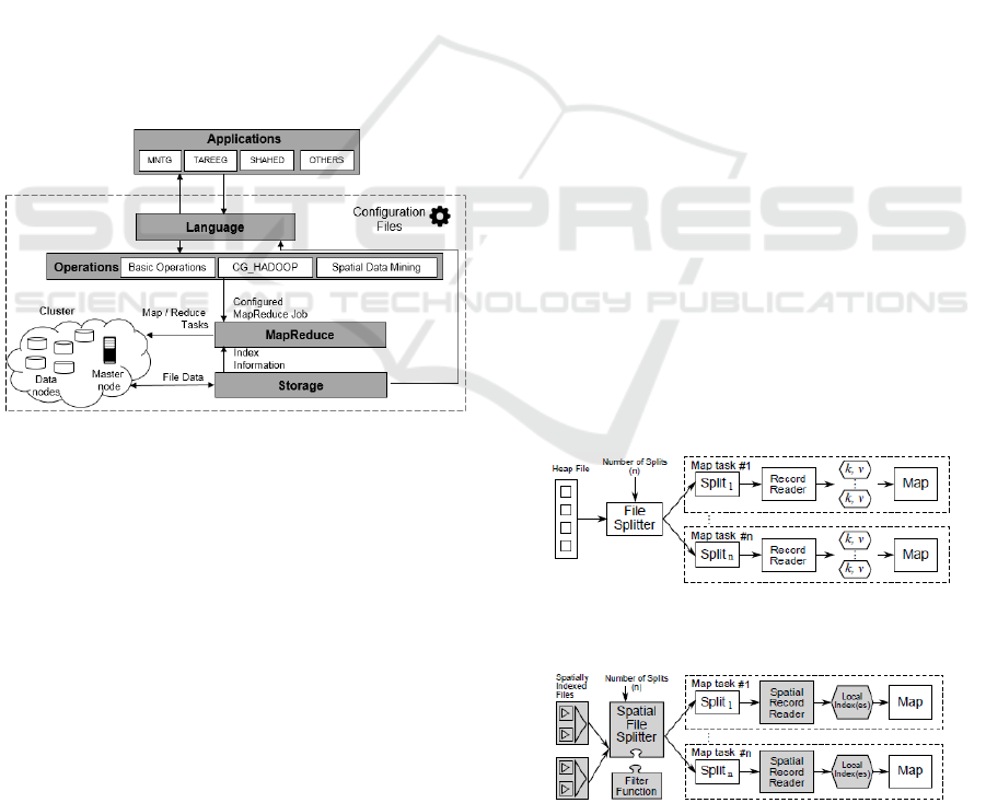
SpatialHadoop comprises four main layers

(Figure 1), namely, language, operations,

MapReduce and storage. All of them execute in a

cluster environment with one master node that breaks

a MapReduce job into smaller tasks, carried out by

slave nodes.

Figure 1: SpatialHadoop high-level architecture.

The Application layer is out from the

SpatialHadoop core, but is fundamental to interact

with users. Among these applications, are:

CG_Hadoop, proposed by Eldawy et al. (2013), is a

suite of scalable and efficient MapReduce algorithms

for various fundamental computational geometry

operations, such as, polygon union, skyline, convex

hull, farthest pair, and closest pair; MNTG, a web-

based road network traffic generator, created by

Mokbel et al. (2014); TAREEG, a MapReduce-based

web service, that uses SpatialHadoop fundamentals

for extracting spatial data from Open Street Map,

proposed by Alarabi et al. (2014); SHAHED, that

uses SpatialHadoop to query and visualize spatio-

temporal satellite data, proposed by Eldawy et al.

(2015).

The language used by SpatialHadoop is Pigeon, a

simple high-level SQL-like language, extended from

Pig Latin. It is compliant with the Open Geospatial

Consortium’s (OGC) simple feature access standard,

which is supported in both open source and

commercial spatial Data Base Management System

(DBMS). Pigeon supports OGC standard data types

including point, linestring and polygon, as well as

OGC standard functions for spatial data.

The operations layer encapsulates the

implementation of various spatial operations with

spatial indexes and the new components in the

MapReduce layer. According to Aji et al. (2013), the

operations layer comprises: basic operations, range

query, k-nearest neighbor (knn) and spatial join;

CG_Hadoop, a suite of scalable and efficient

MapReduce algorithms for various fundamental

computational geometry problems, namely, polygon

union, skyline, convex hull, farthest pair, and closest

pair (Eldawy et al., 2013); and spatial data mining,

operations developed using spatial data mining

techniques.

Similar to Hadoop, the MapReduce layer in

SpatialHadoop (Figure 2) is the query processing

layer that runs MapReduce programs (Eldawy and

Mokbel, 2015). However, contrary to Hadoop where

the input files are non-indexed heap files,

SpatialHadoop supports spatially-indexed input files.

SpatialHadoop enriches traditional Hadoop systems

with two main components: SpatialFileSplitter, an

extended splitter that exploits the global index in

input files to perform early pruning of file blocks not

contributing to answer, and SpatialRecordReader,

which reads a split originating from spatially indexed

input files and exploits the local indexes to efficiently

process it.

Figure 2a: MapReduce in traditional Hadoop (Eldawy and

Mokbel, 2015).

Figure 2b: MapReduce in SpatialHadoop (Eldawy and

Mokbel, 2015).

CLOSER 2017 - 7th International Conference on Cloud Computing and Services Science

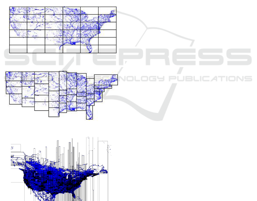
The Storage Layer creates two index layers,

global and local. The global index is applicable on a

cluster’s master node, while local indexes organize

data in each slave node. The SpatialHadoop supports

the main spatial index structures (Eldawy and

Mokbel, 2015): grid file (Figure 3a), a simple flat

index that partitions the data according to a grid, such

that, records overlapping each grid cell are stored in

one file block as a single partition; R-tree (Figure 3b),

in this indexing technique records are not replicated

which causes partitions to overlap; R+-tree (Figure

3c), a variation of the R-tree where nodes at each level

are kept disjoint, while records overlapping multiple

nodes are replicated to each node to ensure efficient

query answering.

Eldawy et al. (2013) developed four more

indexing techniques for SpatialHadoop, namely, Z-

curve, Hilbert curve, Quad tree, and K-d tree, but

these techniques are not as widely used as the others.

Figure 3a: Grid file indexing (Eldawy and Mokbel, 2015).

Figure 3b: R-tree indexing (Eldawy and Mokbel, 2015).

Figure 3c: R+-tree indexing (best viewed in color) (Eldawy

and Mokbel, 2015).

2.3 Related Work

SpatialHadoop was presented in 2013 by Eldawy and

Mokbel (2013) as the first fully-fledged MapReduce

framework with native support for spatial data. In this

article, the authors used a demonstration scenario

created on an Amazon AWS, with 20 node cluster to

compare SpatialHadoop and traditional Hadoop in

three operations, namely, range query, knn and spatial

join. In this paper, as in others, such as, Mokbel et al.

(2014), Alarabi et al. (2014), Eldawy et al. (2015) and

Eldawy et al. (2016), a static computational

environment was used to validate tests. The increase

of data nodes was done in a controlled way, without

automation.

A modular software architecture for processing

big geospatial data in the cloud was presented by

Kramer and Senner (2015). Since the proposed

framework does not distinguish whether the cloud

environment is private or public, a third-party tool –

Ansible – was used to execute provisioning scripts

Finally, in 2016, Das et al. (2016) proposed a

geospatial query resolution framework using an

orchestration engine for clouds. However, the cloud

environment used was private, and no dynamic

allocation of computational resources was performed.

None of these works presents a method to

optimize the use of computational resources, and

reduce financial costs on public cloud providers when

using SpatialHadoop to process big geospatial data.

This paper presents a case study about a cost-

efficient method to process geospatial data on public

cloud providers, optimizing the number of data nodes

in a SpatialHadoop cluster according to dataset size.

3 CLUSTER SIZING

A common uncertainty for Hadoop environment

administrators is how to define the cluster size

infrastructure. In a static environment, like a private

cloud, most of the time the computational resources

are limited and big geospatial data grows faster,

requiring ever more resources. On the other hand, in

public cloud providers, the computational resources

are unlimited, but they come with fees, so it is very

important to define a cost-effective environment.

A twenty-node cluster can be necessary to process

SpatialHadoop queries and operations on a 100Gb

dataset, but is overprovisioned to work on a dataset of

only 5Gb. To solve this problem, a formula to

calculate the quantity of data nodes based on dataset

size is fundamental. Adapting the proposal by

Hadoop Online Tutorial (2016), the following

Cost Optimization on Public Cloud Provider for Big Geospatial Data

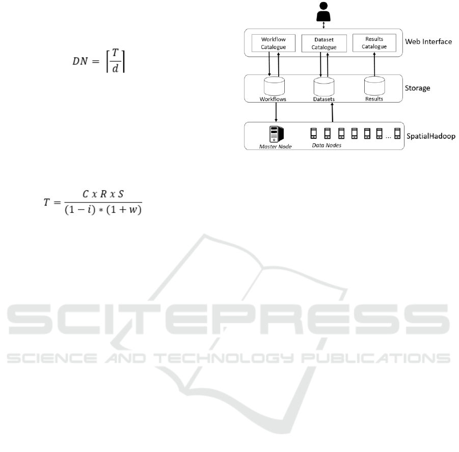
formula can be used to determine the ideal number of

data nodes in a SpatialHadoop environment on public

cloud providers:

(1)

DN represents the total data nodes needed; T is the

total amount of data and d is the disk size in each

node.

It is necessary to calculate T because the total

amount of data used in a SpatialHadoop application

is not only the volume of the dataset. To calculate T,

the following formula can be used:

(2)

C represents the compression rate of the dataset,

required, because SpatialHadoop can work with

compressed files. When no compression is used, the

value must be 1. R is the number of replicas of data in

HDFS and S represents the size of the dataset. The

notation i refers to the intermediate working space

dedicated to temporarily storing results of Map Tasks.

Finally, w represents the percentage of space left

(wasted) to HDFS file system.

To demonstrate the use of these formulas, let us

consider a real Open Street Map dataset of 96Gb of

total size (2.7 billion records) available to download

at http://spatialhadoop.cs.umn.edu/datasets. Without

compression (C = 1), without replication (R = 1),

considering i = 25% and w = 20%, the value obtained

for T is 106.67. Considering that each data node has a

disk with 32Gb (d = 32) it is possible to conclude that

the ideal number of data nodes (DN) is 4.

4 CASE STUDY

To support the method proposed in this paper, a study

case using Open Street Map datasets was executed, in

a cloud environment, built in Amazon AWS provider.

The following sections detail the system architecture,

the datasets used, the tests and the results.

4.1 System Architecture

An architecture composed of three layers, namely

Web Interface, Storage and SpatialHadoop (Figure

4), was created to support the tests environment and

the proposed method.

Figure 4: System Architecture Overview.

The Web Interface Layer is a user-friendly

interface to receive inputs and to show results. In this

layer, the user selects an available dataset (or uploads

one if it is new) using the “Dataset Catalogue”. The

workflow to be executed is loaded or created through

the “Workflow Catalogue”. A workflow contains

information about queries and operations to be

executed and file index type (Grid, R-Tree or R+-

Tree). Results are available in “Results Catalogue”.

The Storage Layer stores all datasets available, the

workflows used, and the results saved after

application execution.

The SpatialHadoop Layer is the core layer. It is

responsible for provisioning the SpatialHadoop

cluster with one master node and n data nodes. The

quantity of data nodes is defined based on dataset

size, as shown in Section 3. After provisioning the

cluster, this layer indexes the dataset (based on user

choice in the Web Interface layer), processes queries

and operations, and saves the results file back in the

Storage Layer.

4.2 Open Street Maps Datasets

The OpenStreetMap (OSM) is a project for

geographic information that has a world map built by

volunteers. The project is open data and can be used

for any purpose.

The OSM files are available on Planet.osm web

site (http://wiki.openstreetmap.org/wiki/Planet.osm)

and the files used in this research are accessible on

SpatialHadoop Datasets website

(http://spatialhadoop.cs.umn.edu/datasets). The file

format is XML and can be downloaded in a

compacted way for convenience.

The datasets considered in our case study are

presented in Table 1. The Lakes’ dataset contains

boundaries of lakes in the world in a 2.7 GB

CLOSER 2017 - 7th International Conference on Cloud Computing and Services Science

compacted file with about 8.4M records. A larger

dataset contains the boundaries of all buildings

around the world – 6 GB in compacted size, and

comprising 115M records. These files were

previously uploaded to Amazon S3, and are available

publicly on the URIs https://s3.amazonaws.com

/spatial-hadoop/input/lakes.bz2 and https://s3

.amazonaws.com/spatial-hadoop/input/buildings.

bz2, respectively.

Table 1: Datasets and their features.

Dataset

Size

Compacted

Records

Lakes

9.0 GB

2.7 GB

8.4

million

Buildings

26.0 GB

6 GB

115

million

4.3 Tests and Results

A SpatialHadoop environment was built using

Amazon AWS EMR to test the proposed method.

Although all three layers of the system architecture –

Web Interface, Storage and SpatialHadoop – were

allocated on a cloud provider, the focus of this test

scenario – performance and cost – was specifically

carried out on the SpatialHadoop layer.

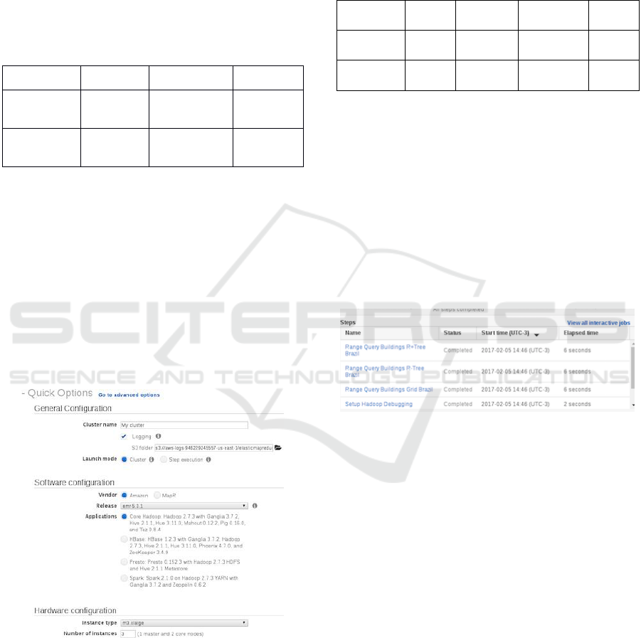
Figure 5 shows the Amazon Web Interface. For

our tests we used the Amazon interface to configure

parameters and execute the scripts.

Figure 5: Amazon Configuration Interface.

Table 2 presents the instances configurations used

to run the tests on Amazon AWS. The master node is

responsible for the cluster management and requires

more memory than datanodes. For the case study, the

master node has 15 GiB memory and 2 SSDs with 80

GiB each. The price per hour for this configuration is

US$ 0.42. The data nodes are responsible for the

spatial data processing. They have 7.5 GiB memory

and 2 SSDs with 40 GiB each. The price per hour for

each node is US$ 0.21.

Table 2: Instances Configurations on Amazon AWS.

Function

vCPU

Memory

Disk

(SSD)

Price

(US$)

Master

2x 80 Gb

0.42 /

hour

Data

Node

7.5

2x 40 Gb

0.21 /

hour

The clusters created for tests comprise one master

node and the quantity of data nodes based on the

formula shown in Section 3. With C = 1, R = 3, i =

25% and w = 20%, 1 data node was required for the

small dataset and 2 data nodes for the big one.

Once parameters were defined in the Web

Interface Layer and the dataset was stored in the

Storage Layer, the SpatialHadoop Layer was

configured to execute the steps (scripts). Each step

was configured with the Amazon Web Interface

(Figure 6). We defined the script and received the

results.

Figure 6: Steps on Amazon Web Interface.

The steps executed were:

• Provisioning Cluster: a defined request is sent to

the cloud provider with the number and type of master

node and data nodes. The command used in Amazon

AWS Command Line Interface (CLI) is:

aws emr create-cluster \

--applications Name=Hadoop \

--bootstrap-actions

'[{"Path":"s3://scripts-nuvem/install-

shadoop-uber.sh","Name":"Instalar

SpatialHadoop"}]' \ --ec2-attributes

'{"KeyName":"acesso-aws",

"InstanceProfile":"EMR_EC2_DefaultRole"

,"SubnetId":"subnet-55f01169",

"EmrManagedSlaveSecurityGroup":"sg-xx",

"EmrManagedMasterSecurityGroup":"sg-

xx"}' --service-role EMR_DefaultRole \

--enable-debugging \ --release- label

emr-5.1.0 --log-uri 's3n://aws-logs-2-

us-east- 1/elasticmapreduce/' \--name

Cost Optimization on Public Cloud Provider for Big Geospatial Data

'geo-cluster' \--instance-groups

'[{"InstanceCount":1,"InstanceGroupType

":"CORE","InstanceType":"c4.xlarge","Na

me":"Core instance group -

2"},{"InstanceCount":1,"InstanceGroupTy

pe":"MASTER","InstanceType":"c4.2xlarge

","Name":"Master instance group -

1"}]' \ --region us-east-1

• Transfer Dataset: copies an existing dataset

from Storage Layer to Data nodes.

• Index Dataset: applies the user-defined index

type to dataset. The AWS CLI command to index a

dataset using Grid is:

aws emr add-steps --cluster-id j-xx \

--steps '[{"Args":["index","s3://dados-

spatial/sports.bz2", "s3://dados-

spatial/sports.index","shape:osm","sind

ex:grid", "-overwrite"],

"Type":"CUSTOM_JAR", "ActionOnFailure":

"CONTINUE","Jar":"/usr/lib/hadoop/spati

alhadoop-2.4-uber.jar",

"Properties":"","Name":"Index"}]'

• Queries and Operations: executes the user-

defined queries and operations. The following AWS

CLI command was used to execute a KNN query:

aws emr add-steps --cluster-id j-xx \

--steps '[{"Args":["knn","s3://dados-

spatial/sports.index", "s3://dados-

spatial/sports-knn.txt", "point:-

15.763372,-47.8700677", "k:1000",

"shape:osm", "-overwrite"],

"Type":"CUSTOM_JAR","ActionOnFailure":"

CONTINUE", "Jar":"/usr/lib/hadoop/

spatialhadoop-2.4-uber.jar",

"Properties":"","Name":"KNN"}]'

• Save Results: saves the result file – usually a text

file – on Storage Layer to be accessed by user.

• Turn-off Cluster: to avoid waste of

computational resources and financial costs, all the

cluster (master node and data nodes) are turned off

unless some stickiness parameter was defined by the

user.

Table 3 presents the runtime of each task in a test

environment. The values represent an average of 3

executions for each dataset. The queries – KNN and

Range Query – and the indexing type Grid were

chosen randomly, and could be changed by any query

or operation and indexing type.

The indexing task is very important to ensure the

SpatialHadoop high performance. Note that the index

process takes up most of the time, but subsequently

the queries are done very quickly.

Table 3: Time measured in each task.

Task

Small Dataset

(seconds)

Large Dataset

(seconds)

Provisioning Cluster

300

420

Transfer Dataset

120

Index Dataset

600

3540

KNN

Range Query

Save Results

Turn-off Cluster

100

164

TOTAL Time

1080

4260

Given the cost of the cluster to support the Small

Dataset (1 master node and 1 data node) as US$

0.63/hour, the total cost to process these two queries

was US$ 0.19. For the cluster to support the large

dataset (comprising 1 master node and 2 data nodes),

the cost per hour is US$ 0.84, and the cost of

processing these queries is US$ 0,99.

If this cluster was created without considering the

dataset’s size – and other parameters defined in the

formula – it would be necessary to consider the

largest dataset available to ensure that any query or

operation could be executed in this cluster.

Considering all datasets available to download on the

SpatialHadoop webpage, the largest dataset – an

OSM file with 137Gb of size and 717M records about

road networks represented as individual road

segments – would require a cluster comprising 1

master node and 6 data nodes. The total cost of this

cluster would be US$ 1.68 per hour and running the

small dataset (18 minutes) would cost US$ 0.50,

costing 263% more than was really needed.

Analysing all datasets available in SpatialHadoop

webpage, and considering the scenario and

parameters defined in our test environment (C = 1, R

= 3, i = 25% and w = 20%), only 7 out of a total of 33

datasets need more than 1 data node to be executed.

On the other extreme, only 1 dataset needs a 6-node

cluster. Processing any other datasets will waste

computational resources if the proposed formula is

not applied.

5 CONCLUSION AND FUTURE

WORKS

The enormous volume of geographic data, produced

daily, through voluntary geographic information

systems, satellite imaging, and other systems, is

classified as Bigdata, or more specifically,

GeoBigdata. To process this geo big data, spatial

cloud computing, comprising several frameworks,

has been presented as a viable tool. In the framework

CLOSER 2017 - 7th International Conference on Cloud Computing and Services Science

that concerns our work, SpatialHadoop has the

infrastructure to process geographic databases, and

many tools have been developed for operations, joins,

and indexing in geodatabases.

Cloud computing provides infrastructure to

process big geospatial data that needs high

performance but requires a computational

infrastructure that can be expensive, when working

on public cloud providers. With this, it is necessary to

use a cost-efficient method to avoid wasting

computational resources and increases in financial

costs.

The method proposed in this paper and

demonstrated by the case study presented, achieves

the goal of supporting a SpatialHadoop environment

on public cloud providers, while avoiding the waste

of computational resources. The formula to define the

number of data nodes was validated in the case study

and about 263% of the cost was econimized.

As future works we suggest optimizations on

performance that can be obtained using task nodes –

for job processing only - and data nodes together. In

this way, it is possible to apply scalability in

SpatialHadoop applications based on user-defined

threads, mainly in indexing task, that demands

powerful computing. Others applications can also be

tested, like SpatialSpark and ISP-MC.

REFERENCES

Ahmed, Elmustafa Sayed Ali, and Rashid A. Saeed. "A

Survey of Big Data Cloud Computing Security."

International Journal of Computer Science and

Software Engineering (IJCSSE) 3.1 (2014): 78-85.

Akdogan, Afsin. Cost-efficient partitioning of spatial data

on cloud. Big Data (Big Data), 2015 IEEE International

Conference on. IEEE, 2015.

Alarabi, L., Eldawy, A., Alghamdi, R., & Mokbel, M. F.

(2014, June). TAREEG: a MapReduce-based web

service for extracting spatial data from OpenStreetMap.

ACM SIGMOD international conference on

Management of data. ACM.

Das, J., Dasgupta, A., Ghosh, S. K., & Buyya, R. A

Geospatial Orchestration Framework on Cloud for

Processing User Queries. In IEEE International

Conference on Cloud Computing for Emerging

Markets, 2016.

Distributed System Archicteture. Hadoop cluster size.

[Online]. Available from: https://0x0fff.com/hadoop-

cluster-sizing/ 2016.10.26.

Eldawy, A., Li, Y., Mokbel, M. F., & Janardan, R. (2013,

November). CG_Hadoop: computational geometry in

MapReduce. The 21st ACM SIGSPATIAL

International Conference on Advances in Geographic

Information Systems.

Eldawy, A., Mokbel, M. F., Alharthi, S., Alzaidy, A.,

Tarek, K., & Ghani, S. (2015, April). Shahed: A

mapreduce-based system for querying and visualizing

spatio-temporal satellite data. In 2015 IEEE 31st

International Conference on Data Engineering (pp.

1585-1596). IEEE.

Eldawy, Ahmed, and Mohamed F. Mokbel. "A

demonstration of SpatialHadoop: an efficient

mapreduce framework for spatial data." Proceedings of

the VLDB Endowment 6.12 (2013): 1230-1233.

Eldawy, Ahmed, and Mohamed F. Mokbel. "Pigeon: A

spatial mapreduce language." 2014 IEEE 30th

International Conference on Data Engineering.

Eldawy, Ahmed, and Mohamed F. Mokbel.

"Spatialhadoop: A mapreduce framework for spatial

data." 2015 IEEE 31st International Conference on

Data Engineering. IEEE, 2015.

Eldawy, Ahmed, Louai Alarabi, and Mohamed F. Mokbel.

"Spatial partitioning techniques in SpatialHadoop."

Proceedings of the VLDB Endowment 8.12 (2015).

Eldawy, Ahmed, M. Mokbel, and Christopher Jonathan.

"HadoopViz: A MapReduce framework for extensible

visualization of big spatial data." IEEE Intl. Conf. on

Data Engineering (ICDE). 2016.

Eldawy, Ahmed. "SpatialHadoop: towards flexible and

scalable spatial processing using mapreduce."

Proceedings of the 2014 SIGMOD PhD symposium.

ACM, 2014.

Hadoop Online Tutorial. Formula to calculate NDFS nodes

storage. [Online]. Avilable from:

http://hadooptutorial.info/ formula-to-calculate-hdfs-

nodes-storage/ 2016.11.03.

Joshi, Pramila. "Cloud Architecture for Big Data."

International Journal of Engineering and Computer

Science. 2015.

Krämer, Michel, and Ivo Senner. "A modular software

architecture for processing of big geospatial data in the

cloud." Computers & Graphics 49 (2015): 69-81.

Leong, L., Petri, G., Gill, B., Dorosh, M. The Gartner Magic

Quadrant for Cloud Infrastructure as a Service,

Worldwide. [Online]. Available from:

https://www.gartner.com/doc/reprints?id=1-2G2O5FC

&ct=150519. 2016.11.02.

Mell, Peter, and Tim Grance. "The NIST definition of cloud

computing." (2011).

Mokbel, M. F., Alarabi, L., Bao, J., Eldawy, A., Magdy, A.,

Sarwat, M., ... & Yackel, S. (2014, March). A

demonstration of MNTG-A web-based road network

traffic generator. In 2014 IEEE 30th International

Conference on Data Engineering (pp. 1246-1249).

IEEE.

Qu, Chenhao, Rodrigo N. Calheiros, and Rajkumar Buyya.

"Auto-scaling Web Applications in Clouds: A

Taxonomy and Survey." arXiv preprint

arXiv:1609.09224 (2016).

Sagiroglu, Seref, and Duygu Sinanc. "Big data: A review."

Collaboration Technologies and Systems (CTS), 2013

International Conference on. IEEE, 2013.

Cost Optimization on Public Cloud Provider for Big Geospatial Data

Ward, Jonathan Stuart, and Adam Barker. "Undefined by

data: a survey of big data definitions." arXiv preprint

arXiv:1309.5821 (2013).

Yang, C., Goodchild, M., Huang, Q., Nebert, D., Raskin,

R., Xu, Y., and Fay, D. (2011). Spatial cloud

computing: how can the geospatial sciences use and

help shape cloud computing?. International Journal of

Digital Earth, 4(4), 305-329.

Yang, C., Goodchild, M., Huang, Q., Nebert, D., Raskin,

R., Xu, Y., & Fay, D. (2011). Spatial cloud computing:

how can the geospatial sciences use and help shape

cloud computing?. International Journal of Digital

Earth, 4(4), 305-329.

Zhang, Q., Cheng, L., Boutaba, R. (2010). Cloud

computing: state-of-the-art and research challenges.

Journal Internet Service Application, 1, 7-8.

CLOSER 2017 - 7th International Conference on Cloud Computing and Services Science