The Impact of Memory Dependency on Precision Forecast
An Analysis on Different Types of Time Series Databases
Ricardo Moraes Muniz da Silva, Mauricio Kugler and Taizo Umezaki
Nagoya Institute of Technology, Department of Computer Science and Engineering,
Showa-ku, Gokiso-cho, 466-8555, Nagoya, Japan
Keywords: Time Series Forecast, ARIMA, ARFIMA, Memory Dependency.
Abstract: Time series forecasting is an important type of quantitative method in which past observations of a set of
variables are used to develop a model describing their relationship. The Autoregressive Integrated Moving
Average (ARIMA) model is a commonly used method for modelling time series. It is applied when the data
show evidence of nonstationarity, which is removed by applying an initial differencing step. Alternatively,
for time series in which the long-run average decays more slowly than an exponential decay, the
Autoregressive Fractionally Integrated Moving Average (ARFIMA) model is used. One important issue on
time series forecasting is known as the short and long memory dependency, which corresponds to how
much past history is necessary in order to make a better prediction. It is not always clear if a process is
stationary or what is the influence of the past samples on the future value, and thus, which of the two
models, is the best choice for a given time series. The objective of this research is to have a better
understanding this dependency for an accurate prediction. Several datasets of different contexts were
processed using both models, and the prediction accuracy and memory dependency were compared.
1 INTRODUCTION
Time series forecasting is one of the most important
types of quantitative models in which past
observations of same variables are collected and
analyzed to develop a model describing their
underlying relationship (Aryal and Wang, 2003).
These models have been used to forecast various
phenomena in many fields, such as agriculture,
economics, environment, tourism and meteorology.
These methods are constantly being improved
and adapted for each particular context in order to
obtain a better prediction of future events (Khashei
and Bijari, 2011).
One example of such adaptations is the classic
case of long and short memory dependence, which
corresponds to how much past history is necessary
in order to make a better prediction, i.e. the
correlation between the data and the model
parameters, which can deviate along time
(Gourieroux and Monfort, 1997).
When modelling a time series, a commonly used
method is the Autoregressive Integrated Moving
Average (ARIMA) model, which is a generalization
of the Autoregressive Moving Average (ARMA)
model.
These methods are applied in the cases where
data show evidence of short memory nonstationarity,
which can be removed by an initial differencing. The
model is generally referred to as an ARIMA(p,d,q)
model, where p, d and q are non-negative integers
that correspond to the order of the autoregressive,
integrated and moving average parts of the model,
respectively.
Alternatively, for modelling time series in the
presence of long memory dependency, the
Autoregressive Fractionally Integrated Moving
Average (ARFIMA) model is used (Granger and
Joyeux, 1980; Hosking, 1984). The ARFIMA(p,d,q)
model generalizes the ARIMA model by allowing
non-integer values of the differencing parameter d.
The main objective of the model is to explicitly
account for long term correlations in the data. It is
useful to model time series in which deviations for
the long-run mean decay more slowly than an
exponential decay.
In this research, we identify the short and long
dependence of ARIMA and ARFIMA models,
estimate their parameters and compare their
forecasting performance in different types of
Silva, R., Kugler, M. and Umezaki, T.
The Impact of Memory Dependency on Precision Forecast - An Analysis on Different Types of Time Series Databases.
DOI: 10.5220/0006203405750582
In Proceedings of the 6th International Conference on Pattern Recognition Applications and Methods (ICPRAM 2017), pages 575-582
ISBN: 978-989-758-222-6
Copyright
c
 2017 by SCITEPRESS – Science and Technology Publications, Lda. All rights reserved
575

databases in order to know the better model for each
different scenario.
The paper is organized as follows. In Section 2,
we briefly present some background on the
mentioned models. The methodology of this
research is discussed in Section 3, and Section 4
present experimental results. Finally the conclusions
are presented in Section 5.
2 BACKGROUND
The particular details of the aforementioned models
in the analysis of correlation and memory
dependency are described in details as follows.
2.1 ARIMA
The ARIMA method is one of the most important
and widely used linear time series models. The
popularity of ARIMA model is due to its statistical
properties as well as the well-known Box-Jenkins
methodology (Box and Jenkins, 1976) in the model
building process. It is an important forecasting
approach that goes through model identification,
parameter estimation and model validation. The
main advantage of this method relies on the
accuracy over a wider domain of series.
The model is based on a linear combination of
past values (AR components) and errors (MA
components). Mathematically, the ARIMA predicted
value 

is given by:


=

(

)

(
1+
(

)


)
(1)
where  is the order of differencing, 

is the error, 
is the lag operator, 
(

)
is given by:

(

)
=1−

−



− … −



(2)
where  are the parameters of the AR terms on the
polynomial of order , and 
(

)
is given by:

(

)
=1+

+



+ … 



(3)
where  indicate the parameters of the MA terms on
the polynomial of order .
In this model, a nonstationary time series is
differentiated  times until it becomes stationary,
where  is an integer. Such series are said to be
integrated of order , denoted 
(

)
, with the non-
differentiated 
(
0
)
being the option for stationary
series. Is important to notice that many series exhibit
too much dependence to be 
(
0
)
but are not 
(
1
)
. In
these cases, there is a persistence in the
observations, which requires the use of prediction
methods that take into consideration the slowly
decaying autocorrelations, among which is the
ARFIMA model (Contreras-Reyes and Palma, 2013;
Dickey and Fuller, 1979), which will be explained
further in this section.
2.1.1 Auto-Correlation Function (ACF)
There are two phases to the identification of an
appropriate ARIMA model (Box and Jenkins, 1976):
changing the data, if necessary, into a stationary
time series and determining the tentative model by
observing the behaviour of the autocorrelation and
partial autocorrelation functions.
A time series is considered stationary when it
does not contain trends, that is, it fluctuates around a
constant mean (Hosking, 1984). The autocorrelation
coefficient 

measures the correlation between a set
of observations and a lagged set of observation in a
time series:


=
∑(


−̅
)(


−̅
)


∑(


−̅
)



(4)
where 

is the 

sample of the stationary time
series, 

is the sample from  time period ahead
of  and 
is the mean of the stationary time series.
Box and Jenkins suggest the number of pairs
used to calculate the autocorrelation to be no more
than =4. The sample autocorrelation coefficient


is an initial estimate of ρ

.
2.1.2 Partial Auto-Correlation Function
(PACF)
The estimated Partial Autocorrelation Function
(PACF) is used as a guide, along with the estimated
ACF, in choosing one or more ARIMA models that
might fit the available data.
The objective of the partial autocorrelation
analysis is to measure how

and 

are related.
The equation that gives a good estimate of the partial
autocorrelation 

is:

,
=


−
∑

,




1−
∑

,




(5)
where:

,
=
,
−
,

,

,
=

(6)
2.1.3 Stationary Process
The ARIMA model is intended to be used with
stationary time series, i.e. time series in which their
ICPRAM 2017 - 6th International Conference on Pattern Recognition Applications and Methods
576

statistical properties are constant over time
(Hosking, 1984).
The stationarity of a time series can be evaluated
by accuracy measures, such as the Sum Squared
Error (SSE) or the Mean Absolute Percentage Error
(MAPE), given by:
SSE =
∑(


−

)



(7)
MAPE =


∑







×100%


(8)
where N is the number of predicted values and 

and 

are, respectively, the 

actual and predicted
values.
However, is not always clear if a given process is
stationary or not. In this cases, the ARFIMA model
can be used, since can work with nonstationary time
series (Granger, 1989).
2.2 ARFIMA
The ARFIMA model is one of the best-known
classes of long-memory models (Contreras-Reyes
and Palma, 2013). It provide a solution for the
tendency to over-differentiate stationary series that
exhibit long-run dependence, allowing a continuum
of fractional differencing parameter −0.5 <  <
+0.5 (Souza, and Smith, 2004; Zhang, 2003).
This generalization to fractional differences
makes possible to handle processes that are neither

(
0
)
nor 
(
1
)
, to test for over-differentiation, and to
model long-run effects that only die out at long
horizons (Baum, 2000; Fildes and Makridakis,
1995).
The ARFIMA model is described as follow:

(

)(
1−
)



=
(

)


(9)
where:
(
1−
)

=
(
−
)


(
−
)(
+1
)


(10)
The stochastic process 

is both stationary and
invertible if all the roots of 
(

)
and 
(

)
present
<0.5.
In recent years, studies about long memory
dependency have received the attention of
statisticians and mathematicians. This phenomenon
has grown rapidly and can be found in many fields,
such as hydrology, chemistry, physics, economics
and finances (Boutahar and Khalfaoui, 2011;
Moghadam and Keshmirpour, 2011).
2.2.1 Long and Short Memory Dependency
A times series with long memory dependence is
often referred to the concept of fractional
integration, since there is the necessity to expand the
differentiation order, spreading the use of past
values.
An stationary time series can be considered a
short memory process, since the AR(p) model has
infinite memory, as all the past values of 

are
embedded in 

. However, the effects on the past
values, rapidly decreasing geometrically to near
zero. The MA(q) model uses a memory of order q;
consequently, the effects of the moving average
component also diminish fast (Palma, 2007;
Anderson, 2000).
In comparison, the autocorrelation of the
ARFIMA model has a hyperbolical decay, in
contrast to the faster, geometric decay of a stationary
ARMA process. Consequently, a series with long
memory dependency has an autocorrelation function
that decline more slowly than the decrease exhibited
on the short memory process (Hurvich and Ray,
1995; Geweke and Porter-Hudak, 1983).
This was observed in other works, in which some
datasets present better accuracy with the ARIMA
model with short memory (Shitan et al., 2008),
while other datasets perform better with the
ARFIMA model with long memory (Amadeh et al.,
2013).
Thus, an ARFIMA process may be predictable at
longer horizons. A survey of long memory models
applied in economics and finance is given by Baillie
(Baillie, 1996).
2.2.2 Spectral Density
Inverting the ARFIMA model described in equation
(7) gives:


=
(
1−
)

(

(

)
)


(

)


(11)
After the parameter estimation, the short-run
effects are obtained by setting =0 in equation
(11), and describe the behaviour of the fractionally
differenced process
(
1−
)



. The long-run effects
use the estimated value of d from equation (9), and
describe the behaviour of the fractionally integrated


.
Granger and Joyeux (Granger and Joyeux, 1980)
motivate the use of ARFIMA models by noting that
their implied spectral densities for >0 are finite
except at null frequency, whereas stationary ARMA
models have finite spectral densities at all
frequencies. The ARFIMA model is able to capture
The Impact of Memory Dependency on Precision Forecast - An Analysis on Different Types of Time Series Databases
577

the long-range dependence, which cannot be
expressed by stationary ARMA models.
The two models imply different spectral
densities for frequencies close to zero when >0.
The spectral density of the ARMA model remains
finite, but is pulled upward by the model's attempt to
capture long-range dependence. The short-run
ARFIMA parameters can capture both low-
frequency and high-frequency components in the
spectral density (Sowell, 1992; Priestley, 1981). In
contrast, the ARMA model confounds the long-run
and short-run effects.
3 METHODOLOGY
In this study, the standard modelling time series
methodologies ARIMA and ARFIMA have been
employed. These models require the following steps
in order to be trained: identification, parameters
estimation, validation, modelling and prediction.
Specific details are described on the literature
(Granger and Joyeux, 1980; Box and Jenkins, 1976).
The modelling tools for time series forecast were
developed in-house using MATLAB, given special
attention to the monitoring of some particular
aspects of each dataset.
Although both methods have been widely
applied in several different contexts and long and
short memory dependency analysed for independent
datasets, the forecasting process still requires both
methods to be applied and their performance
compared in order to determine the best model for
each case (Chan, 1992; Chan 1995).
Thus, the objective of this research is to have a
better understanding of the level of dependency and
how much historical data is necessary for an
accurate prediction, considering the follow aspects:
 spectral density and statistical properties;
 differences on stationary series behaviour;
 impact of long and short memory dependency;
This aspects were analysed on several different
datasets described in the following section.
3.1 Datasets
The datasets used in the experiments were obtained
from the UCI Machine Learning Repository
(Lichman, M., 2013) and Sugar Price Database from
the Brazilian Stock Market BM&F Bovespa (BM&F
Bovespa, 2016).
Datasets of a wide variety of contexts were
selected in order to generalize the analysis of the
different models to several different scenarios. The
datasets are listed in Table 1, while the details of
each dataset are shown in Tables 2-9.
Table 1: Time Series Datasets.
Dataset Table
Sugar Price Database 2
Greenhouse Gas Observing Network 3
Electricity Load Diagrams 4
Individual Household Power Consumption 5
Combined Cycle Power Plant 6
Solar Flare 7
Istanbul Stock Exchange 8
Dow Jones Index 9
Table 2 describes the Ibovesp Stock Market
database, which tracked the evolution of the price of
50kg sugar bag from November 2003 to
May 2009.
Table 2: Sugar Price Database.
Datasets Characteristics Time Series
Number of Instances 3346
Number of Attributes 3
Associated Task Classification / Regression
Area Business
The dataset in Table 3 contains values of
greenhouse gas (GHG) concentrations at 2921 grid
cells in California, created using simulations of the
Weather Research and Forecast model with
Chemistry (Lucas et al., 2015).
Table 3: Greenhouse Gas Observing Network.
Datasets Characteristics Multivariate, Time Series
Number of Instances 2921
Number of Attributes 5232
Associated Task Regression
Area Physical
Table 4 describes a datasets of electricity
consumption from 370 points per clients from 2011
to 2014 period.
Table 4: Electricity Load Diagrams.
Datasets Characteristics Time Series
Number of Instances 370
Number of Attributes 140256
Associated Task Regression / Clustering
Area Computer
The dataset in Table 5 contains measurements of
electric power consumption in one household with a
one-minute sampling rate over a period of almost 4
years. It also contains different electrical quantities
and sub-metering values.
ICPRAM 2017 - 6th International Conference on Pattern Recognition Applications and Methods
578

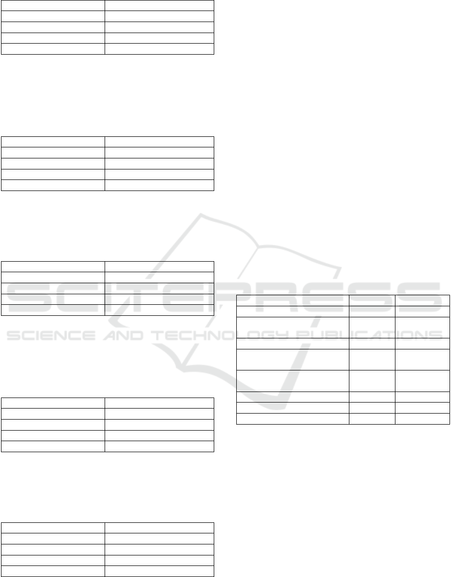
Table 5: Individual Household Power Consumption.
Datasets Characteristics Multivariate, Time Series
Number of Instances 2075259
Number of Attributes 9
Associated Task Regression / Clustering
Area Physical
Table 6 describes a dataset of points collected
from a combined cycle power plant over 6 years
(2006-2011), when the plant was set to work with
full load (Tüfekci, 2014; Kaya et al., 2012).
Table 6: Combined Cycle Power Plant.
Datasets Characteristics Multivariate
Number of Instances 9568
Number of Attributes 4
Associated Task Regression
Area Computer
The dataset in Table 7 contains the number of
solar flares of 3 potential classes that occurred in a
24 hour period.
Table 7: Solar Flare.
Datasets Characteristics Multivariate
Number of Instances 1389
Number of Attributes 10
Associated Task Categorical
Area Physical
Table 8 details a datasets that includes returns of
the Istanbul Stock Exchange with seven other
international indexes, from June 2009 to February
2011 (Akbilgic et al., 2013).
Table 8: Istanbul Stock Exchange.
Datasets Characteristics Multivariate, Time Series
Number of Instances 536
Number of Attributes 8
Associated Task Classification / Regression
Area Business
Finally, the dataset described in Table 9 contains
weekly data from the Dow Jones Industrial Index.
(Brown et al., 2013).
Table 9: Dow Jones Index.
Datasets Characteristics Time Series
Number of Instances 750
Number of Attributes 16
Associated Task Classification / Clustering
Area Business
As shown in Tables 2-9, the selected datasets
present a wide range of instances and attributes, as
well as different areas of application.
3.2 Time Series Modelling Procedures
The standard approach to temporal series prediction
is to apply different methods (e.g. ARIMA and
ARFIMA), and compare their performances in order
to select the method with the minimal average
forecasting error.
In this paper, not only the performance of the
methods but also the influence of the use of short
and long memory dependency was evaluated for
each different datasets in several scenarios.
4 EXPERIMENTS AND RESULTS
Considering the several different types of databases,
the analysis was made in order to show the impact of
memory dependency on the forecasting accuracy in
different areas. In all cases, the models were
simulated with both methodologies (ARIMA and
ARFIMA). Table 10 shows the best fit (p, q and d)
for both model in each dataset.
Table 10: Best fit for each model (p, q, d).
Database ARIMA ARFIMA
Sugar Price Database (1, 1, 3) (2, 0.23, 4)
Greenhouse Gas
Observing Network
(1, 0, 2) (2, 0.17, 1)
Electricity Load Diagrams (2, 1, 1) (3, 0.5, 2)
Individual Household
Power Consumption
(4, 0, 1) (1, -0.34, 5)
Combined Cycle
Power Plant
(3, 1, 5) (1, 0.47, 3)
Solar Flare (1, 1, 6) (2, 0.33, 1)
Istanbul Stock Exchange (2, 0, 1) (3, 0.29, 5)
Dow Jones Index (3, 0, 5) (4, -0.42, 3)
In a typical ARIMA process, the patterns of ACF
and PACF indicate the structure of the model. A
long autocorrelation imply that the process is non-
linear with time variance, implying that the
properties of memory dependency between two
distance observations are still visible.
In order to maintain the correlation between the
observed values and their lag, and consequently the
influence of the past value in the current
observation, the value of the lag is suggested to be
no greater than 4. This value, however, was
exceeded in some cases, as shown in Table 11.
The Impact of Memory Dependency on Precision Forecast - An Analysis on Different Types of Time Series Databases
579

Table 11: Memory Dependency based on the
Autocorrelation Function.
Database Lag
Sugar Price Database -
Greenhouse Gas Observing Network Exceeded
Electricity Load Diagrams -
Individual Household Power Consumption -
Combined Cycle Power Plant Exceeded
Solar Flare -
Istanbul Stock Exchange Exceeded
Dow Jones Index Exceeded
In some time series, these larger lag values
indicate that the ACF do not decay exponentially
over time, but rather decay much slower and show
no clear periodic pattern.
The memory dependency can also be estimated
by observing the statistical properties of the data,
such as MAPE and SSE, as demonstrated by Alireza
and Ahmad (Alireza and Ahmad, 2009). In this
work, the percentage average absolute error (PAAE)
for both models was calculated and the results
shown in Table 12.
Table 12: Percentage of Average Absolute Error.
Database ARIMA ARFIMA
Sugar Price Database 31.67% 32.23%
Greenhouse Gas
Observing Network
18.47% 17.26%
Electricity Load Diagrams 10.98% 11.56%
Individual Household
Power Consumption
15.64% 17.12%
Combined Cycle Power Plant 21.05% 19.22%
Solar Flare 9.68% 10.42%
Istanbul Stock Exchange 29.12% 28.41%
Dow Jones Index 30.05% 29.85%
When ARFIMA was used on data with small
variance, the observed PAAE was low. By contrast,
when ARIMA was used on data with high variance,
the observed PAAE was high. This is because the
accumulative error per sampling will be greater on a
high variance data with smaller order of integration.
The analysis performed so far enable the
comparison of the forecast precision (high or low),
as well as how much dependency each dataset
presents (short or long). It must be noticed that some
of the datasets have particular behaviour or external
influences (e.g. stock market) that affect the quality
of the prediction. The results are shown in Table 13.
Table 13: Memory Dependency and Forecast Precision.
Database
Dependenc
y
Precision
Sugar Price Database Short *Low
Greenhouse Gas Observing
Network
Long High
Electricity Load Diagrams Short *High
Individual Household
Power Consumption
Short High
Combined Cycle
Power Plant
Long *High
Solar Flare Short *High
Istanbul Stock Exchange Long *Low
Dow Jones Index Long *Low
Some datasets, marked with *, denoted an
unexpected behaviour when considering the
properties of the time series. For instance, it is
usually considered that a linear series with small
number of samples and short dependency will result
in a high precision (Yule, 1926). However, the
obtained results show that this is not always the case
(e.g. Sugar Price).
The databases related with stock market
(Istanbul Stock Exchange and Dow Jones Index)
have a long memory dependency, but present low
accuracy. This is due to the fact that these are highly
volatile processes and are difficult to predict with
linear modelling tools (Engle and Smith, 1999). In
the other hand, the Solar Flare dataset is a classic
example of seasonal behaviour, but the
measurements need to be carefully made on a
correct window of time.
Datasets related with electricity and power
consumption usually have a linear behaviour,
achieving high precision (Taylor et al., 2006). The
Electricity Load Diagrams dataset, however, has a
very large number of attributes, resulting in a large
variance. Although it presents short dependency
characteristics, this dataset requires a careful
selection of the most relevant attributes on the
quantification of electricity consumption.
On the Combined Cycle Power Plant, the data
was acquired only at full-load times. Thus, the data
presents characteristics of long memory dependence,
leading to a high forecast precision.
5 CONCLUSIONS
This paper analyses the effects of memory
dependency in several different time series datasets
and the influence on the forecast accuracy. Two
commonly used methods, ARIMA and ARFIMA,
were used for this analysis.
ICPRAM 2017 - 6th International Conference on Pattern Recognition Applications and Methods
580

For some datasets, the ARIMA model presented
better forecast results (smaller PAAE) when
compared with the ARFIMA model. This might be
because the ARFIMA model is based on a long
memory process, while some datasets are less
affected by external activities and other processes.
However, that does not imply that having more
historical data will always result in a better forecast.
In a linear model scenario, independently of the used
statistical properties and the monitoring of memory
dependency values, the data itself should still be
carefully analysed in order to achieve an accurate
prediction.
This indicates that it is not always clear how
much impact the past values have on the
accumulative error and what is their influence in the
future values. A possible solution for this is to
increase the lag in the ACF and observe the effect of
the prediction accuracy of future values. Different
time windows can also be used to achieve a better
fitting, as observed in the course of this study.
Specific pre-processing operations can be
applied to each dataset in order to reduce the
accumulative error, but only in situations in which a
clear objective exists.
The obtained results motivate the development
of a combined methodology compatible with both
fractional and integer integration values along the
time series prediction, in order to account for short
and long memory dependencies. Future work also
include the use of more and larger datasets in order
to further understand the memory dependency
effects on time series forecasting.
ACKNOWLEDGEMENTS
The first author is supported by the Ministry of
Education, Culture, Sports, Science and Technology
(MEXT), Government of Japan.
REFERENCES
Aryal, D. R., Wang, Y., 2003. Neural Network
Forecasting of the Production Level of Chinese
Construction Industry. Journal of Comparative
International Management, vol. 6, no. 2, pp. 45-64.
Khashei M., Bijari M., 2011. A New Hybrid Methodology
for Nonlinear Time Series Forecasting. Modelling and
Simulation in Engineering, Article ID 379121, 5
pages.
Gourieroux, C. S., Monfort, A., 1997. Time Series and
Dynamic Models, Cambridge University Press.
Granger, C. W. J., Joyeux, R., 1980. An introduction to
long memory time series models and fractional
differencing. Journal of Time Series Analysis, vol. 1,
no. 1, pp. 15-29.
Hosking, J. R. M., 1984. Modelling Persistence in
Hydrological Time Series using Fractional
Differencing. Water Resources Research, vol. 20, no.
12, pp. 1898-1908.
Box, G. E. P., Jenkins, G. M., 1976. Time series analysis:
forecasting and control, Holden Day. San Francisco,
1
st
edition.
Contreras-Reyes, J. E., Palma, W. 2013. Statistical
analysis of autoregressive fractionally integrated
moving average models in R. Computational
Statistics, vol. 28, no. 5, pp. 2309-2331.
Dickey, D. A., Fuller, W. A., 1979. Distribution of the
estimators for autoregressive time series with unit
root. Journal of the American Statistical Association,
vol. 74, no. 366, pp. 427-431.
Granger, C. W. J., 1989. Combining forecasts - Twenty
years later. Journal of Forecasting, vol. 8, no. 3, pp.
167-173.
Souza, L. R., Smith, J., 2004. Effects of temporal
aggregation on estimates and forecasts of fractionally
integrated processes: a Monte-Carlo study.
International Journal of Forecasting, vol. 20, no. 3,
pp. 487-502.
Zhang, G. P., 2003. Time series forecasting using a hybrid
ARIMA and neural network model. Neurocomputing,
vol. 50, pp. 159-175.
Baum, C. F., 2000. Tests for stationarity of a time series.
Stata Technical Bulletin, vol. 57, pp. 36-39.
Fildes, R., Makridakis, S., 1995. The impact of empirical
accuracy studies on time series analysis and
forecasting, International Statistical Review, vol. 63,
no. 3, pp. 289-308.
Boutahar, M., Khalfaoui, R., 2011. Estimation of the long
memory parameter in non stationary models: A
Simulation Study, HAL id: halshs-00595057.
Moghadam, R. A., Keshmirpour, M., 2011. Hybrid
ARIMA and Neural Network Model for Measurement
Estimation in Energy-Efficient Wireless Sensor
Networks, In ICIEIS2011, International Conference
on Informatics Engineering and Information Science.
Springer, vol. 253, pp. 35-48.
Palma, W., 2007. Long-Memory Time Series: Theory and
Methods, Wiley-Interscience, John Wiley & Sons.
Hoboken.
Anderson, M. K., 2000. Do long-memory models have
long memory? International Journal of Forecasting,
vol. 16, no. 1, pp. 121-124.
Hurvich C. M., Ray, B. K., 1995. Estimation of the
memory parameter for nonstationary or noninvertible
fractionally integrated processes. Journal of Time
Series Analysis, vol. 16, no. 1, pp. 17-42.
Geweke, J., Porter-Hudak, S., 1983. The estimation and
application of long-memory time series models.
Journal of Time Series Analysis, vol. 4, no. 4, pp. 221-
238.
The Impact of Memory Dependency on Precision Forecast - An Analysis on Different Types of Time Series Databases
581

Shitan, M., Jin Wee P.M., Ying Chin, L., Ying Siew, L.,
2008. Arima and Integrated Arfima Models for
Forecasting Annual Demersal and Pelagic Marine Fish
Production in Malaysia, Malaysian Journal of
Mathematical Sciences, vol. 2, no. 2, pp. 41-54.
Amadeh, H., Amini, A., Effati, F., 2013. ARIMA and
ARFIMA Prediction of Persian Gulf Gas-Oil F.O.B.
Iranian Journal of Investment Knowledge, vol. 2, no.
7, pp. 213-230.
Baillie, R. T., 1996. Long memory processes and
fractional integration in econometrics. Journal of
Econometrics, vol. 73, no. 1, pp. 5-59.
Sowell, F., 1992. Modelling long-run behaviour with the
fractional ARIMA model. Journal of Monetary
Economics, vol. 29, no. 2, pp. 277-302.
Priestley, M. B., 1981. Spectral Analysis and Time Series,
Academic Press. London.
Chan, W. S., 1992. A note on time series model
specification in the presence outliers, Journal of
Applied Statistics, vol. 19, pp. 117–124.
Chan, W. S., 1995. Outliers and financial time series
modelling: a cautionary note. Mathematics and
Computers in Simulation, vol. 39, no. 3-4, pp. 425-
430.
Lichman, M., 2013. UCI Machine Learning Repository
[http://archive.ics.uci.edu/ml]. Irvine, CA: University
of California, School of Information and Computer
Science.
Brazilian Stock Market BM&F Bovespa. Accessed on
April 2016. [http://www.bmfbovespa.com.br]
Lucas, D. D., Yver Kwok, C., Cameron-Smith, P., Graven,
H., Bergmann, D., Guilderson, T. P., Weiss, R.,
Keeling, R., 2015. Designing optimal greenhouse gas
observing networks that consider performance and
cost. Geoscientific Instrumentation, Methods and Data
Systems, vol. 4, no. 1, pp. 121-137.
Tüfekci, P., 2014. Prediction of full load electrical power
output of a base load operated combined cycle power
plant using machine learning methods. International
Journal of Electrical Power & Energy Systems, vol.
60, pp. 126-140.
Kaya, H., Tüfekci, P., Gürgen, S. F., 2012. Local and
Global Learning Methods for Predicting Power of a
Combined Gas & Steam Turbine, In ICETCEE2012,
International Conference on Emerging Trends in
Computer and Electronics Engineering, pp. 13-18.
Akbilgic, O., Bozdogan, H., Balaban, M. E., 2013. A
novel Hybrid RBF Neural Networks model as a
forecaster, Statistics and Computing, vol. 24, no. 3, pp.
365-375.
Brown, M. S., Pelosi, M. J., Dirska, H., 2013. Dynamic-
Radius Species-Conserving Genetic Algorithm for the
Financial Forecasting of Dow Jones Index Stocks. In
MLDM2013, 9th International Conference on
Machine Learning and Data Mining in Pattern
Recognition, Springer, pp. 27-41.
Alireza, E., Ahmad J., 2009. Long Memory Forecasting of
Stock Price Index Using a Fractionally Differenced
Arma Model. Journal of Applied Sciences Research,
vol. 5, no. 10, pp. 1721-1731.
Yule, G. U., 1926. Why do we sometimes get nonsense-
correlations between time series? A study in sampling
and the nature of time-series. Journal of the Royal
Statistical Society, vol. 89, no. 1, pp. 1-63.
Engle, R. F., Smith A. D., 1999. Stochastic permanent
breaks. Review of Economics and Statistics, vol. 81,
no. 4, pp. 553-574.
Taylor, J. W., Menezes, L. M., McSharry, P. E., 2006. A
comparison of univariate methods for forecasting
electricity demand up to a day ahead, International
Journal of Forecasting, vol. 22, no. 1, pp. 1-16.
ICPRAM 2017 - 6th International Conference on Pattern Recognition Applications and Methods
582