Extracting Latent Behavior Patterns of People from Probe Request Data:
A Non-negative Tensor Factorization Approach
Kaito Oka
1
, Masaki Igarashi
2
, Atsushi Shimada
3
and Rin-ichiro Taniguchi
2
1
Graduate School of Information Science and Electrical Engineering, Kyushu University, Fukuoka, Japan
2
Faculty of Information Science and Electrical Engineering, Kyushu University, Fukuoka, Japan
3
Faculty of Arts and Science, Kyushu University, Fukuoka, Japan
Keywords:
Probe Request, People Flow, Location Information, Non-negative Tensor Factorization, Data Mining.
Abstract:
Although people flow analysis is widely studied because of its importance, there are some difficulties with
previous methods, such as the cost of sensors, person re-identification, and the spread of smartphone applica-
tions for collecting data. Today, Probe Request sensing for people flow analysis is gathering attention because
it conquers many of the difficulties of previous methods. We propose a framework for Probe Request data
analysis for extracting the latent behavior patterns of people. To make the extracted patterns understandable,
we apply a Non-negative Tensor Factorization with a sparsity constraint and initialization with prior knowl-
edge to the analysis. Experimental result showed that our framework helps the interpretation of Probe Request
data.
1 INTRODUCTION
The observation of people flow is studied widely
using various methods such as monitoring systems
using stereo cameras (Heikkil
¨
a and Silv
´
en, 2004),
laser-range-finder-based human tracking (Jung et al.,
2014), and mining from data collected by Location-
Based Services (LBSs) data (Hsieh et al., 2012).
However, these methods all have some disadvan-
tages. People flow analysis using cameras/laser-
range-finders has difficulty tracking a person between
different sensors because personal ID information is
not collected directly. In addition, these sensors are
expensive and difficult to install in new environments.
People flow analysis using LBS has a poor data cov-
erage. That is, if we want to analyze people flow at
a certain location, the quantity of data depends on the
percentage of people passing that location that use the
application. For instance, the Foursquare dataset
1
in
New York City has 3,112 users in it, but the data con-
sists of 0.036% of the population in New York City.
Currently, another approach for people flow anal-
ysis is gathering attention: Probe Request sensing
(Schauer et al., 2014) (Fukuzaki et al., 2014). A Probe
1
Foursquare Dataset https://sites.google.com/site/
yangdingqi/home/foursquare-dataset/ Accessed 22 August
2016
Request is a Wi-Fi connection request packet from
a Wi-Fi device to nearby Access Points (APs). The
Probe Request sensing method overcomes the disad-
vantages of the other methods above. First, we can
collect the identified flows of each person by sens-
ing Probe Requests because the packet includes the
device ID (MAC address). Second, we can collect a
large amount of data because Wi-Fi devices transmit
Probe Requests periodically while the Wi-Fi is turned
on. In other words, we can collect data from Wi-Fi
devices whether or not they have installed a particular
application. Finally, Probe Request sensors are small
and cheap, so we can easily install the sensing sys-
tem in a new environment. (Table 1 summarizes this
comparison.)
Since Probe Request sensing method has high
coverage of data, dimension reduction is effective for
analyzing the data. However, some dimension reduc-
tion methods, such as Principal Component Analysis,
are not helpful for interpreting the data. The reason is
that they lose the original meaning of each axis (e.g.
users, location, etc.) and we can hardly understand
what each axis mean after the reduction.
In this paper, we propose a framework for analyz-
ing people flow via Probe Request sensing. Specif-
ically, we apply a Non-negative Tensor Factoriza-
tion (NTF), which is a kind of dimension reduction
method that does not lose the original meaning of
Oka, K., Igarashi, M., Shimada, A. and Taniguchi, R-i.
Extracting Latent Behavior Patterns of People from Probe Request Data: A Non-negative Tensor Factorization Approach.
DOI: 10.5220/0006193901570164
In Proceedings of the 6th International Conference on Pattern Recognition Applications and Methods (ICPRAM 2017), pages 157-164
ISBN: 978-989-758-222-6
Copyright
c
 2017 by SCITEPRESS – Science and Technology Publications, Lda. All rights reserved
157

Table 1: Comparison of methods for people flow analysis.
Method
Person tracking
Data coverage Installation
between sensors
Camera Difficult High Difficult
Laser-range-finder Difficult High Difficult
LBS Easy Low Easy
Probe Request sensing Easy High Easy
each axis, to extract the latent behavior patterns of
people. Additionally, we use a sparsity constraint and
prior knowledge to make the extracted patterns more
understandable. The latent behavior patterns indicate
what people do in the sensing field. For instance,
group A could have lunch, those in group B study, and
those in group C do both. Experimental results show
that the proposed framework helps the interpretation
of people’s behavior from Probe Request data.
2 RELATED WORK
2.1 People Flow Analysis by Probe
Request Sensing
Schauer et al. analyzed people flow through a secu-
rity check at a German airport to show the correlation
between the estimated number of people by sensing
Probe Request and the real number of people that pass
the security check (Schauer et al., 2014). They in-
stalled two Probe Request sensors: one before people
passed through the security check and another after
the check. The experiment was held for 16 days, and,
for each day, they calculated Pearson’s correlation of
the data. The experimental results showed that cor-
relation value r was 0.75 on average when they used
RSSI and received time information.
Fukuzaki et al. developed a system that analyzes
pedestrian flow using their own Probe Request sen-
sors (Fukuzaki et al., 2014). The system handles
Probe Request data using hash values of the MAC
addresses instead of the original MAC addresses to
ensure the anonymity of Wi-Fi device users. The au-
thors installed the system in a real environment: a
two day graduation work exhibition at Osaka Electro-
Communication University. They analyzed the peo-
ple flow during the exhibition in terms of numbers
of people and how long they stayed at each location,
and created an origin-destination table that shows how
many people moved from where to where. They con-
cluded that they can analyze the rough tendency of a
pedestrian flow with the system.
2.2 Application of Tensor Factorization:
Prediction and Recommendation
Sahebi et al. proposed a tensor factorization approach
called Feedback Driven Tensor Factorization for
modeling student learning processes and predicting
student performances (Hsieh et al., 2016). They de-
scribed a three-dimensional tensor that shows whether
student A passed or failed quiz Q on a certain attempt,
and factorized it into another three-dimensional ten-
sor and matrix. The three-dimensional tensor calcu-
lated from the factorization indicates students’ pro-
cess of acquiring knowledge (e.g., what pointers do
in programming) by solving quizzes, and the ma-
trix shows which knowledge is needed for answer-
ing quizzes. Their approach showed higher accuracy
than other approaches for the task of predicting stu-
dent performance.
Zheng et al. developed a mobile recommendation
system that helps those wishing to sightsee or dine
in a large city (Zheng et al., 2012). If we send a
certain location as a query, their system returns rec-
ommended activities at that location. To the con-
trary, if we send a certain activity as a query, their
system returns recommended locations for the activ-
ity. They proposed PARAFAC (Bro, 1997) based ten-
sor factorization with some prior knowledge terms for
this recommender system. They confirmed that their
approach outperformed other baseline approaches in
terms of a recommendation task by comparing the ac-
curacy of estimating the null values in the original ten-
sor.
3 PROPOSED FRAMEWORK
In this section, we explain the proposed framework
for extracting the latent behavior patterns of people
from Probe Request data. In order to extract behav-
ior patterns that indicates the staying times of peo-
ple that are sensitive to time and place, we com-
pose a three-dimensional tensor that shows ”who”(the
user) stayed ”where”(the location) for ”how long”(a
value in hours) ”when”(time in hours). Here, ”who,”
”where,” and ”when” are indices of the tensor, and
ICPRAM 2017 - 6th International Conference on Pattern Recognition Applications and Methods
158

”how long” is the element. We then factorize this ten-
sor into three matrices: a user latent factor matrix, lo-
cation latent factor matrix, and time latent factor ma-
trix. Note that we can reduce the dimension of data
without losing the original meaning of each axis (user,
location, and time), by applying NTF. (We further ex-
plain the proposed NTF in detail in Section 4.)
3.1 Probe Request Data and
Preprocessing
As we note in Section 1, a Probe Request is a Wi-
Fi connection request packet from a Wi-Fi device to
nearby APs. Wi-Fi devices transmit Probe Requests
periodically with an interval of about 30–120 s (de-
pending on the device) (Fukuzaki et al., 2014). By
sensing Probe Requests from Wi-Fi devices, espe-
cially smartphones, we get MAC address, which iden-
tify each device, and the distance between the sen-
sor and device as indicated by the Received Signal
Strength Indicator (RSSI) value. Thus, we can an-
alyze the flow of people carrying Wi-Fi devices by
tracing an identified device by the history of sensors
it has passed or remained near.
In this work, we use sensors called AIBeacons
2
to collect Probe Request data. Each AIBeacon asyn-
chronously uploads the collected data to the database
server about three times per minute. When the AIBea-
con uploads Probe Request data, it uses the hash
values of the MAC addresses instead of the original
data to ensure the private information of Wi-Fi device
users are not leaked. In accordance with (Fukuzaki
et al., 2014), we call this hashed value an Anonymous
MAC (AMAC) address. Table 2 shows an example of
the data we obtain from the database server. Note that
the unit of RSSI is not dBm due to the specification
of AIBeacon, RSSI is not a negative value, and lower
RSSI indicates shorter distance. In addition, some
Wi-Fi devices transmit Probe Requests with random-
ized MAC addresses, so tracing such devices is im-
possible. Therefore, we removed such data from our
analysis.
Remember that we can estimate whether a device
is near a distributed sensor because the RSSI is a
barometer of distance between a sensor and a device.
In other words, we can obtain the location of a user
at a certain time. From this location information, we
can calculate ”who”(the user) stayed ”where”(the lo-
cation) for ”how long”(a value in hours, the element
of the tensor) ”when”(time in hours), which composes
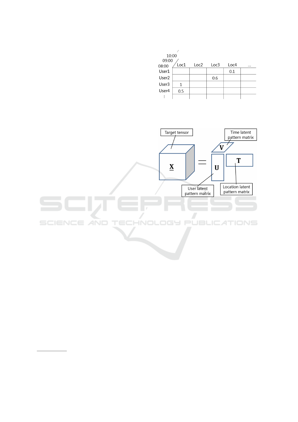
the three-dimensional tensor, as shown in Figure 1.
2
AIBeacon, http://aibeacon.jp/ (Japanese website), Ac-
cessed 22 August 2016
Figure 1: Three-dimensional tensor data. The value indi-
cates the time (hours) that the user stayed at a particular
location. For instance, User4 stayed at Loc1 for 0.5 hours
between 08:00–09:00 h.
Figure 2: Non-negative Tensor Factorization (NTF).
3.2 NTF with Sparsity Constraint and
Initialization with Prior Knowledge
As mentioned in the introduction, our goal is to ex-
tract the latent behavior patterns of people, which are
helpful for data interpretation. To achieve this goal,
we propose the use of NTF (Figure 2) with a sparsity
constraint and prior knowledge. The sparsity con-
straint clarifies which factor is important for some
users, locations, and times. Prior knowledges (e.g.,
8:00 h is breakfast time, Restaurant A is open from
08:00 h to 19:00 h, etc.) also help our understanding
of the data. We use prior knowledges by initializing
the place and time latent factor matrices. By setting
initial value according to prior knowledges, we can
not only examine whether extracted patterns fit to the
given prior, but also discover unexpected patterns.
From the decomposed matrices, we can obtain
which users are strongly affected by a certain fac-
tor. Figure 3 shows an example of the proposed NTF.
For instance, the user group indicated by the black
frame is affected by the breakfast and studying fac-
tors. These users should have breakfast and study in
the sensing field. Similarly, the user group indicated
by the green frame is affected by the lunch factor and
should have lunch.
Extracting Latent Behavior Patterns of People from Probe Request Data: A Non-negative Tensor Factorization Approach
159

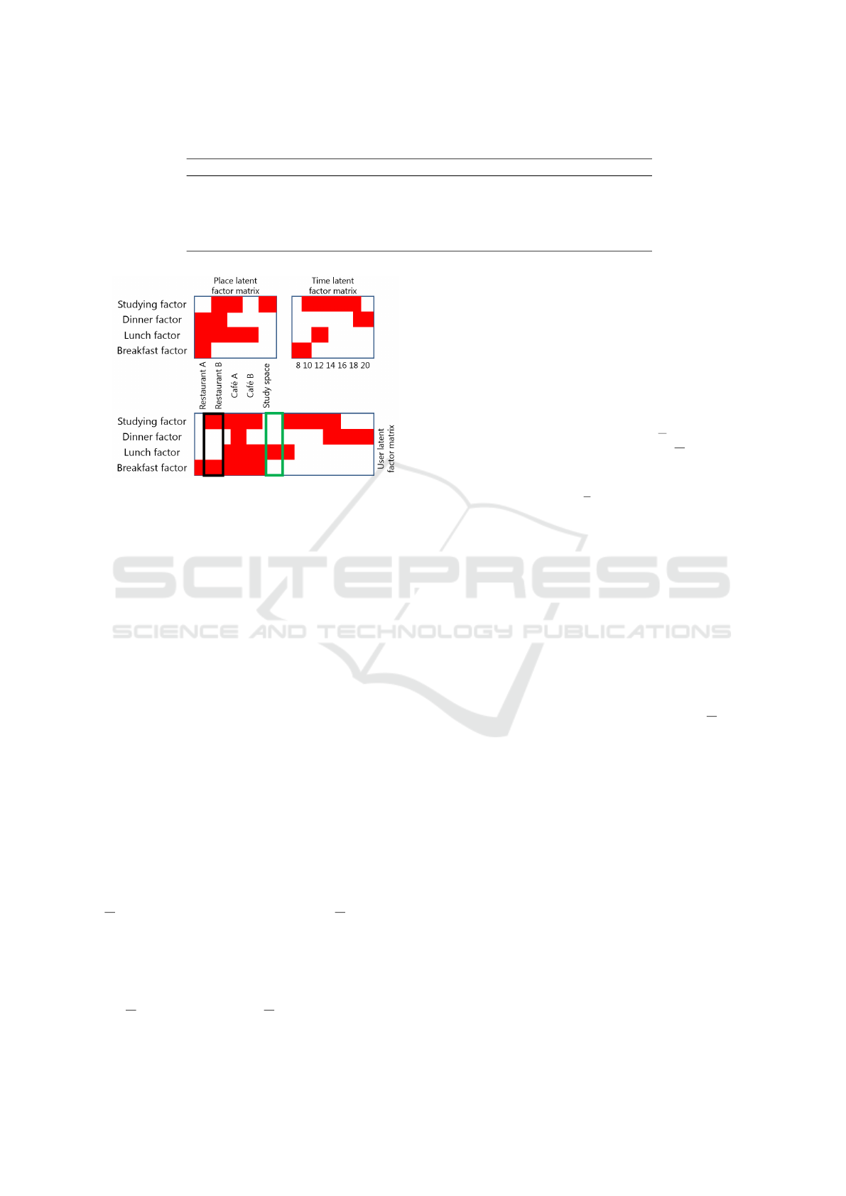
Table 2: Example of data from a database server.
AMAC address RSSI Randomized flag Unixtime[s] Sensor ID
203xx...xxe5c8 94 0 1443884406 10000011
265xx...xx9e5a 62 0 1443884408 1000000C
89cxx...xx9adc 85 1 1443884409 1000000D
.
.
.
.
.
.
.
.
.
.
.
.
.
.
.
Figure 3: Example results. The meaning of each factor is
defined by prior knowledge.
4 NTF FOR EXTRACTING
UNDERSTANDABLE
PATTERNS
In this section, we explain the details of the NTF with
a sparsity constraint and prior knowledge, which are
the most important contributions of this paper. As we
mentioned in Section 3.2, we use NTF to decompose
the data into three matrices that indicate which fac-
tor is important for some users, locations, and times.
First, we show the basis of Tensor Factorization in
Section 4.1. We next explain the formulation of the
non-negativity and sparsity constraints in Section 4.2.
Finally, the algorithm and initialization with prior
knowledge are explained in Section 4.3.
4.1 Formulation of Tensor Factorization
Let the target three-dimensional L × M × N tensor be
X. Here, we consider factorizing this X into three
matrices: L × K user latent factor matrix U, M × K
location latent factor matrix T, and N × K time la-
tent factor matrix V. Note that K is a parameter
that determines the number of factors. If we obtain
three matrices that completely describe original ten-
sor X, each element x
lmn
in X and each latent pattern
vector u
l
= [u
l1
, . . . , u
lK
]
T
, t
m
= [t
m1
, . . . ,t
mK
]
T
, and
v
n
= [v
n1
, . . . , v
nK
]
T
fulfill the following equation.
x
nml
=
K
∑
k=1
u
lk
t
mk
v
nk
(1)
That is, x
nml
is expressed by a multiplication of three
latent pattern vectors: the latent pattern vectors of
user l, location m, and time n. Using Equation 1, we
formulate cost function C
TF
(U, T, V). Tensor factor-
ization is then equal to calculating the U, T, and V
that minimize C
TF
(U, T, V). Here, D
X
is the set of
indices that point to non-null elements in X.
C
TF
(U, T, V) =
∑
(l,m,n)∈D
X
(x
lmn
−
K
∑
k=1
u
lk
t
mk
v
nk
)
2
(2)
Equation 2 is the fundamental cost function of the ten-
sor factorization, which is the same as the standard
PARAFAC tensor decomposition (Bro, 1997).
4.2 Non-negativity and Sparsity
Constraint
If we allow negative values in the calculated matrices,
factors may cancel each other out by subtraction or
multiplication of the negative values. This is not de-
sirable for understanding the meaning of each factor.
Thus, we added non-negativity constraint to Equation
2, i.e., u
lk
,t
mk
, v
nk
≥ 0. Under this constraint, X can
be expressed as a summation of factors so that we can
understand what each vector means.
If t
lk
, u
mk
, and v
nk
each indicate the strength of the
effect of the kth factor, it is easier to understand the
extracted latent pattern. To distinguish clearly which
factor is important for each user, location, and time,
we introduce a sparsity constraint. Concretely, we add
an L1-norm regularization term to the cost function
in Equation 2. Let the cost function be C
TF−sparse
,
calculated as
C
TF−sparse
(U, T, V) = C
TF
(U, T, V)
+ λ(kUk
1
+ kTk
1
+ kVk
1
).
(3)
Finally, let
ˆ
U,
ˆ
T, and
ˆ
V be the three matrices that min-
imize the cost function
(
ˆ
U,
ˆ
T,
ˆ
V) = arg min
U,T,V
C
TF−sparse
(U, T, V)
s.t. u
lk
,t
mk
, v
nk
≥ 0 for all l, m, n, k. (4)
ICPRAM 2017 - 6th International Conference on Pattern Recognition Applications and Methods
160

4.3 Algorithm and Initialization with
Prior Knowledge
This section presents the algorithm of the proposed
NTF. Just as (Zheng et al., 2012), the cost function in
Equation 3 is not jointly convex to all variables U, T,
and V, so what we want to obtain is a locally optimal
solution. Note that the cost function in Equation 3 has
an L1-norm regularization term.
In order to obtain a locally optimal solution, our
algorithm uses Forward Backward Splitting (FOBOS)
(Duchi and Singer, 2009) at update step of each pa-
rameters. FOBOS can consider the error function and
L1-norm regularization term separately in the param-
eter update step. In other words, updating parameters
consists of two steps; the first step uses the gradient
of the error function, and the second step uses the L1-
norm regularization term. Our proposed cost function
3 consists of the error function (Equation 2) and the
L1-norm regularization term. Thus, FOBOS effec-
tively works for the proposed cost function.
As we mentioned in Section 3.2, we use prior
knowledge for initialization, which is different from
other standard techniques of NTF. In concrete terms,
we give the initial values for T and V. We also define
the meaning of factors manually in advance to help
our understanding of the extracted user latent factor
matrix. Moreover, we set the following update pa-
rameters: γ
usr
for the user matrix, γ
loc
for the loca-
tion matrix, and γ
time
for the time matrix. By set-
ting γ
loc
, γ
time
< γ
usr
, the calculated matrices keeps the
meaning of the factors. Thus, we can obtain the lo-
cally optimal solution that can be easily understood.
The whole algorithm of the proposed NTF is de-
scribed in Algorithm 1. The gradients of the error
function 2 used in the algorithm is described in Table
3.
Table 3: Gradients for equation 2.
δC
TF
δu
l
=
∑
m,n
(
∑
K
k=1
u
lk
t
mk
v
nk
− x
lmn
)(t
m
◦ v
n
)
δC
TF
δt
m
=
∑
l,n
(
∑
K
k=1
u
lk
t
mk
v
nk
− x
lmn
)(u
l
◦ v
n
)
δC
TF
δv
n
=
∑
l,m
(
∑
K
k=1
u
lk
t
mk
v
nk
− x
lmn
)(u
l
◦ t
m
)
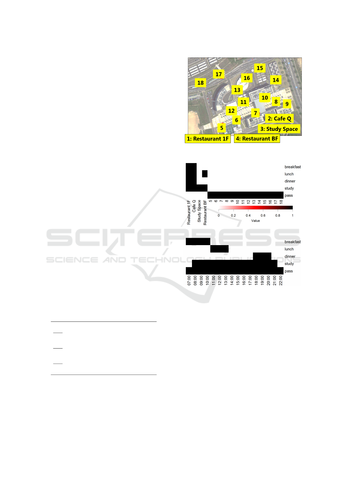
Figure 4: Sensor distribution in the campus.
(a) Place latent factor matrix
(b) Time latent factor matrix
Figure 5: Place and time latent factor matrices initialized by
prior knowledge. Each value is 1 or 0.
5 EXPERIMENT
5.1 Experimental Data
We distributed AIBeacons in the campus, as shown in
Figure 4. Note that locations 1, 2, and 4 are restau-
rants and location 3 is a room for studying. Because
we regard these four locations as important, we put
two sensors each at these locations to collect accurate
data. Other locations are equipped with one sensor
each.
We applied our framework to the data, which
were collected on July 4, 2016, during 07:00–22:00
h. So as to ignore fixed Wi-Fi devices, we re-
Extracting Latent Behavior Patterns of People from Probe Request Data: A Non-negative Tensor Factorization Approach
161

Algorithm 1: Algorithm of proposed NTF.
input : L × M ×N 3-dimensional tensor X
output: L ×K user latent factor matrix U, M × K location latent factor matrix T, and N × K time latent
factor matrix V
1 Initialize the parameters U, T, and V
2 while not convergence do
3 for i = 1 to |D
X
| do
4 Randomly sample (l, m, n) from D
X
5 u
tmp
l
← u
l
, t
tmp
m
← t
m
, v
tmp
n
← v
n
// temporary store
6 Update u
l
← u
l
− γ
usr
δC
TF
δu
l
// first step for error function
7 for k = 1 to K do
8 if u
lk
< 0 then
9 u
lk
← u
tmp
lk
// non-negativity constraint
10 u
lk
← u
lk
− γ
usr
λ // second step for L1-norm
11 if u
lk
< 0 then
12 u
lk
← 0
13 Update t
m
← t
m
− γ
loc
δC
TF
δt
m
// first step for error function
14 for k = 1 to K do
15 if t
mk
< 0 then
16 t
mk
← t
tmp
mk
// non-negativity constraint
17 t
mk
← t
mk
− γ
loc
λ // second step for L1-norm
18 if t
mk
< 0 then
19 t
mk
← 0
20 Update v
n
← v
n
− γ
time
δC
TF
δv
n
// first step for error function
21 for k = 1 to K do
22 if v
nk
< 0 then
23 v
nk
← v
tmp
nk
// non-negativity constraint
24 v
nk
← v
nk
− γ
time
λ // second step for L1-norm
25 if v
nk
< 0 then
26 v
nk
← 0
moved the AMAC addresses that were observed dur-
ing 01:00-05:00 h. In addition, to reduce the com-
putational cost, we sampled 200 users from the total
of 6,824 observed users. Finally, the size of the three-
dimensional tensor was 200 (users) × 16 (hours) × 18
(locations), and consists of 1,079 values. Thus, about
98% of its elements are null values.
5.2 Result
We compared the proposed NTF method (Proposed
NTF) with two baseline methods. One is the NTF
method with no sparsity constraint and no prior
knowledge (Pure NTF), and the other is the NTF
method with a sparsity constraint but no prior knowl-
edge (Sparse NTF). For the Sparse NTF, we set pa-
rameter λ = 0.03. For the Proposed NTF, param-
eter λ = 0.03, and, update parameters were set as
γ
usr
= 0.005 and γ
loc
= γ
time
= 5.0 × 10
−6
. In addi-
tion, in the Proposed NTF, initialization was done by
the matrices in Figure 5. In the initialized place latent
factor matrix shown in Figure 5(a), Restaurant 1F is
open from 08:00 h to 20:30 h and available for study-
ing, so it has the value for the ”breakfast,” ”lunch,”
”dinner,” and ”study” factors. Likewise, the factors
of Cafe Q and Restaurant BF are initialized according
to their opening hours. Other locations (5-18) that do
not seem to be areas where people are stationary have
the ”pass” factor. The time latent factor matrix was
initialized with the matrix shown in Figure 5(b): each
factors has values for the suitable times.
Table 4 shows a comparison of the number of ze-
ros in the factorized matrices, and the recomposition
error indicated by RMSE (Equation 5).
ICPRAM 2017 - 6th International Conference on Pattern Recognition Applications and Methods
162

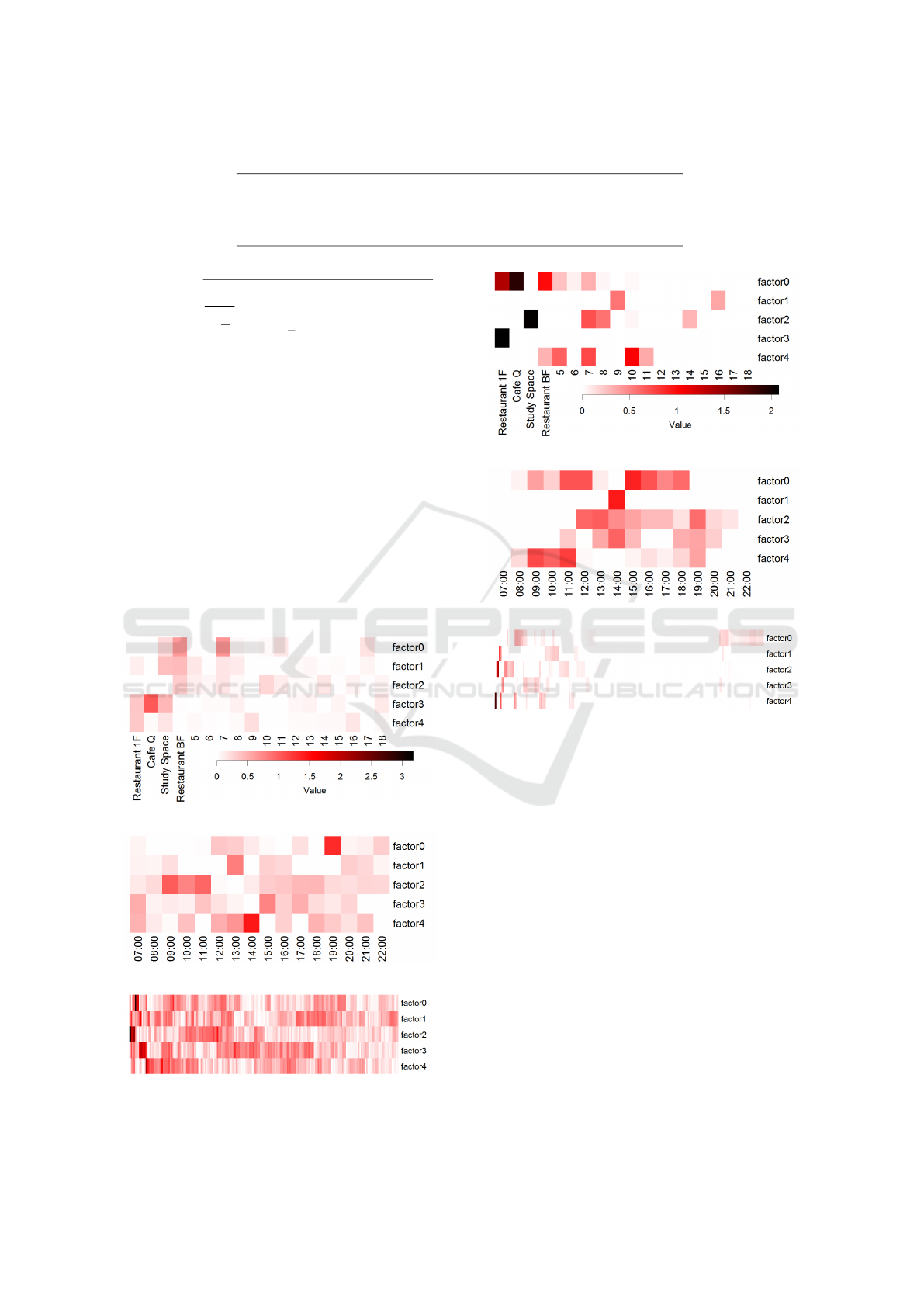
Table 4: Comparison of re-composed error and number of zeros.
Method RMSE Number of zeros (percentage[%])
Proposed NTF 0.0510 832 (71%)
Pure NTF 0.0387 0 (0%)
Sparse NTF 0.0464 924 (79%)
RMSE =
v
u
u
t
1
|D
X
|
∑
(l,m,n)∈D
X
(x
lmn
−
K
∑
k=1
u
lk
t
mk
v
nk
)
2
(5)
Naturally, the more constraints we add, the bigger the
error becomes. However, we can obtain more zeros
with the sparsity constraint, which indicates that we
can understand the data more simply.
Figure 6 and Figure 7 show the latent factor ma-
trices calculated by the Pure NTF and Sparse NTF,
respectively. It is obvious that the results of the
Pure NTF (Figure 6) are not helpful for interpretation.
Compared with the Pure NTF, the results of the Sparse
NTF (Figure 7) seem to be easier to understand. For
example, in the place latent matrix in Figure 7(a), fac-
tor 3 is affected only by Restaurant 1F. Hence, we can
analogize that the meaning of factor 3 is ”Restaurant
1 only,” and the people that are affected by factor 3
only went to Restaurant 1 only on that day.
(a) Place latent factor matrix
(b) Time latent factor matrix
(c) User latent factor matrix
Figure 6: Latent matrices obtained by the Pure NTF.
(a) Place latent factor matrix
(b) Time latent factor matrix
(c) User latent factor matrix
Figure 7: Latent matrices obtained by the Sparse NTF.
Latent factor matrices calculated by the Proposed
NTF are shown in Figure 8. Compared to the Sparse
NTF (Figure 7), we can easily understand the result of
the Proposed NTF because its factors have the clear
meanings. For example, we can say that there are
fewer people who had breakfast than those who had
lunch. Moreover, we can obtain the unexpected pat-
terns from the change from the initialized matrices.
For instance, in the time latent factor matrix shown
in Figure 8(b), the ”pass” factor of 12:00 h has lower
value than other times, which indicates people tend to
stay somewhere at 12:00 h. In addition, in the place
latent factor matrix shown in Figure 8(a), Location 7
is affected by the ”lunch” and ”study” factors after the
factorization, which shows that there are some peo-
ple who stay at Location 7 during lunch and studying
time. What makes our interpretation of the data easier
is the meaning of the factors, which remains after the
factorization.
Extracting Latent Behavior Patterns of People from Probe Request Data: A Non-negative Tensor Factorization Approach
163

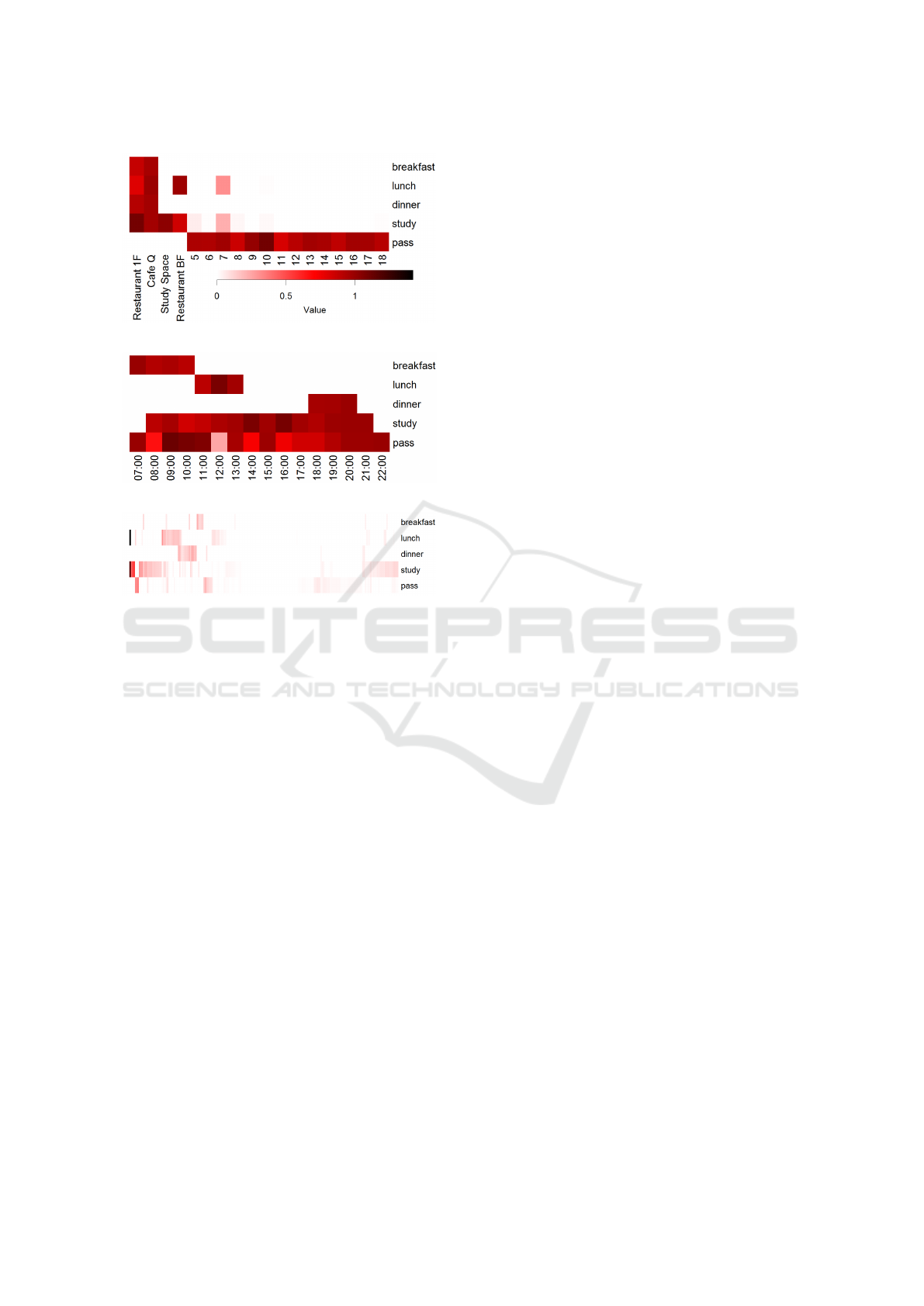
(a) Place latent factor matrix
(b) Time latent factor matrix
(c) User latent factor matrix
Figure 8: Latent matrices obtained by the Proposed NTF.
6 CONCLUSION
We proposed an overall framework for the analysis of
Probe Request data. In order to understand the data
easily, we applied an NTF with a sparsity constraint
and initialization with prior knowledge to the analy-
sis. The experimental results show that our frame-
work helps the interpretation of the Probe Request
data.
For future work, we plan to apply this framework
to real shop data, for which we do not know much
about the people’s behavior patterns. In addition, we
would like to overcome the problem of computational
cost to apply the proposed framework to bigger data.
ACKNOWLEDGEMENTS
We would like to thank AdInte Co., Ltd. for support-
ing our research.
REFERENCES
Bro, R. (1997). Parafac. tutorial and applications. Chemo-
metrics and Intelligent Laboratory Systems.
Duchi, J. and Singer, Y. (2009). Efficient online and batch
learning using forward backward splitting. Journal of
Machine Learning Research.
Fukuzaki, Y., Nishio, N., Mochizuki, M., and Murao, K.
(2014). A pedestrian flow analysis system using wi-fi
packet sensors to a real environment. In ACM Interna-
tional Joint Conference on Pervasive and Ubiquitous
Computing.
Heikkil
¨
a, J. and Silv
´
en, O. (2004). A real-time system for
monitoring of cyclists and pedestrians. Image and Vi-
sion Computing.
Hsieh, H. P., Li, C. T., and Lin, S. D. (2012). Exploiting
large-scale check-in data to recommend time-sensitive
routes. In UrbComp’12, ACM SIGKDD International
Workshop on Urban Computing.
Hsieh, H. P., Li, C. T., and Lin, S. D. (2016). Tensor factor-
ization for student modeling and performance predic-
tion in unstructured domain. In EDM’12, 9th Interna-
tional Conference on Educational Data Mining.
Jung, E. J., Lee, J. H., Yi, B. J., Park, J. Y., Yuta, S., and
Noh, S. T. (2014). Development of a laser-range-
finder-based human tracking and control algorithm for
a marathoner service robot. IEEE/ASME Transactions
on Mechatronics.
Schauer, L., Werner, M., and Marcus, P. (2014). Estimat-
ing crowd densities and pedestrian flows using wi-fi
and bluetooth. In MOBIQUITOUS’14, 11th Interna-
tional Conference on Mobile and Ubiquitous Systems:
Computing, Networking and Services.
Zheng, V. W., Zheng, Y., Xie, X., and Yang, Q. (2012). To-
wards mobile intelligence: Learning from gps history
data for collaborative recommendation. Artificial In-
telligence.
ICPRAM 2017 - 6th International Conference on Pattern Recognition Applications and Methods
164