Open Data Sources for 3D Data Visualisation

Generating 3D Worlds based on OpenStreetMaps Data

Almar Joling

Deltares, Delft, The Netherlands

Keywords: OpenStreetMaps, Procedural Mesh Generation, World Generation, Virtual Worlds, GIS.

Abstract: Georeferenced data is becoming increasingly more available through open source licenses. In this paper, an

approach is explained to build a real-time interactive 3D virtual world using the Unity 3D engine by using

the freely available OpenStreetMaps data. This virtual environment can serve as a base for the visualisations

of spatial and georeferenced data. By making use of OpenStreetMaps this virtual environment can be kept

up to date with changes in the world. This paper provides an introduction to OpenStreetMaps, discusses

some of the challenges and provides examples how to process this data in order to generate a virtual

environment.

1 INTRODUCTION

OpenStreetMaps (OSM) data (OpenStreetMap,

2016) has the advantage of being a single data

source which can provide information about any

location on Earth. Users can edit the maps through

different online tools available on the OSM website

or standalone applications. The size of the database

is continuously increasing (Stats - OpenStreetMap

Wiki, 2016).

Various side projects have also emerged, which

aim to improve the available map data in areas of

need during emergencies or calamity situations. One

of these is the Humanitarian OpenStreetMap Team

project (Hotosm.org, 2016). Many other services and

tools use the OSM data to provide routing

information for GPS devices

(Garmin.openstreetmap.nl, 2016) or smartphones

(Osmand.net, 2016). OSM data is also used for

offline visualisations such as city layout posters

(Paologianfrancesco.com, 2016) and 3D tactile maps

for people who are visually impaired (Kärkkäinen,

2016). Indeed, open and freely available map data

allows the creation of many diverse applications.

This paper describes the results of a research

project aimed at visualising spatial data in a virtual

environment, which is based upon data provided by

OpenStreetMaps. The origin of the visualised spatial

data could come from output of model simulations,

GIS data files or real-time data provided by online

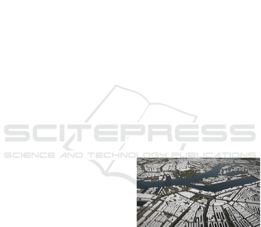
data services. We started with the generation of a 3D

world (Figure 1) based upon OSM data to create a

solid base for adding other data sources, as well as

creating a visual reference point when the spatial

data is viewed. In order to create a realistic

experience, the Unity (Unity, 2016) game engine

version 5.4 is used.

Figure 1: Generated visualisation of the port of Rotterdam,

Netherlands.

2 RELATED WORK

Various tools have been developed or are currently

in development to visualise OSM data in 3D. Some

tools generate their visualisations in a web browser

such as F4Maps (F4map Demo - Interactive 3D

map, 2016), Vizicities (UDST/vizicities, 2016) and

OSMBuildings (Osmbuildings.github.io, 2016).

Joling A.

Open Data Sources for 3D Data Visualisation - Generating 3D Worlds based on OpenStreetMaps Data.

DOI: 10.5220/0006164902510258

In Proceedings of the 12th International Joint Conference on Computer Vision, Imaging and Computer Graphics Theory and Applications (VISIGRAPP 2017), pages 251-258

ISBN: 978-989-758-228-8

251

Other tools are standalone applications, such as

osm2world (Knerr, 2016) and can save 3D model

files, which in turn can serve as an input for other

applications. All of these tools use the same OSM

database as input, and have to process the data in

order to generate the 3D worlds.

Few projects use a game engine to load OSM

data. ActionStreetMap (Actionstreetmap.github.io,

2016) generates 3D worlds in Unity and allows a

player to walk through and interact with the map as

well as saving a scene back to the OSM XML file

format. It also features the ability of dynamic

loading of world elements, which is not present in

our own project.

3 ARCHITECTURE

OSM data can be downloaded from various

websites. One way to acquire this data is by

downloading a data extract based upon

administrative borders such as countries, provinces

and states (download.geofabrik.de, 2016). Another

way is to perform an actual query to receive an

extract of a data set. One such query language is the

OSM Extended API (Xapi - OpenStreetMap Wiki,

2016), which was used in this project. Our query

uses only the bounding box query option, as all data

is potentially useful for 3D visualisation. Therefore

the data of interest is extracted at a later step. The

Xapi query language always returns the latest

version of the dataset, previous versions of nodes

(map elements) are not returned. The API returns

files in the OSM XML format which can then be

used by other software.

3.1 Processing the Data

There are many tools that can operate on OSM files.

A large single XML file is difficult to index for a

real-time application, which is why additional pre-

processing is required before we start generating

world geometry. OSMFilter (Osmfilter -

OpenStreetMap Wiki, 2016) is used to select the

nodes that are interesting in the virtual environment:

land use, buildings, waterways and infrastructure

such as roads, railroads, high voltage towers and

windmills. Some objects, such as windmills, have

been selected for their generality. These objects are

created as Unity prefabs that can easily be placed on

the terrain and do not require extra processing. They

add an extra dimension to the terrain as they are

often landmarks in an area. After filtering, the

command line application ogr2ogr.exe (Gdal.org,

2016) is used to convert the OSM XML file to a

SQLite database. This will automatically categorise

the sources of data in tables with the names equal to

the type of data stored: lines, multilinestrings,

multipolygons and points. Geometry data is stored in

the Well Known Binary (WKB) format.

3.2 Challenges of the OSM Data

Using OSM data does come with potential

challenges when creating visualisations. Although

the amount of data in the database is steadily

growing, many areas in the world are still

incomplete which can leave lots of gaps between

buildings in cities. Aside from that, the actual nature

of OSM has both pros and cons; everyone can edit

the database after making a free account. The

advantage of this is that changes in the real world

are accounted for quickly in the database.

Unfortunately it also means that data can be

incomplete (Figure 2) or mapped incorrectly.

Figure 2: A city which is incompletely mapped.

Tallahassee, USA.

Therefore, certain assumptions in visualisations need

to be made. For example, some of the problems that

have been noticed are nodes with a building tag

which are part of storage underneath a bridge. Or

small wind turbines placed on roofs which in the

generated world become large turbines. This is a

challenge that every 3D OSM visualisation must

handle.

4 TERRAIN GENERATION

All terrain and objects are generated as triangles and

use Unity’s Mesh object to be rendered. In order to

improve performance most of the geometry is

marked as static geometry and aggregated as much

as possible in one single mesh object.

IVAPP 2017 - International Conference on Information Visualization Theory and Applications

252

In this project five elements have been marked as

having significant influence for the visual

representation of the terrain. These are: roads, trees,

buildings, water surfaces and ground textures. Of

course, there are many more man-made objects,

some of which are tagged, but many of these do not

add an extra sense of positional awareness on the

average scale of our map; they are too small and far

away to be seen.

4.1 Terrain Mesh Creation

The terrain is generated using tiles based on the

OSM zoom level 14 (Zoom levels - OpenStreetMap

Wiki, 2016). This was an early design choice based

upon the average expected zoom level of the world,

a trade-off between required tiles and expected map

detail. OSM tiles use a Cartesian coordinate system

based upon EPSG:3857. The actual downloaded

OSM data makes use of the EPSG:4326 (WGS84)

coordinate system.

The elevation of the terrain is based upon the

SRTMv3 (Shuttle Radar Topography Mission, 2016)

global elevation map. This data is freely available

and has accuracy from 30 to 90 meter depending on

the area of interest.

All terrain related information is generated and

rendered per tile using Maperitive (Maperitive.net,

2016). One single tile always represents an OSM tile

at zoom level 14. Terrain is generated by building

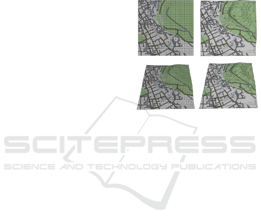
square geometry with a variable number of vertices.

Originally a 32x32 regular grid was used to build

the terrain tiles. But in order to reduce triangle

count, a simple method of Level of Detail (LOD) is

implemented by making use of an error threshold to

determine where to place the vertices. This

technique is loosely based on existing algorithms

(Garland and Heckbert, 1995). The threshold is

configured to be a 15% difference in elevation

between the last vertex and the vertex that is being

processed. When the threshold is exceeded, a new

vertex is inserted at the location and will serve as the

new starting point for the next difference

comparison. Every terrain tile is built using this

algorithm (Figure 3). For convenience, however, all

terrain tiles will have vertices inserted at the four

corner points, such that these will always connect

properly and also guarantees that later tile

tessellation algorithms generate a square exactly the

size of a single OSM tile.

For all the edges of the terrain we store the

vertices in a list. We keep track of these as

neighbouring terrain tiles will need to share the same

vertices at the same location in order to prevent

seams from appearing at the mesh boundaries due to

differences in the elevation.

Neighbouring tiles are quickly determined by

using the OSM coordinates (x -1 or +1 for horizontal

neighbours, y-1 or y+1 for vertical neighbours).

Figure 3: An unoptimised (left) and optimized (right) tile.

When the terrain geometry for a tile has been

processed and all vertices have been created, the

tessellation LibTessDotNet (speps/LibTessDotNet,

2016) library is used to create renderable triangles

using Delaunay triangulation.

This process is repeated three times with

different tolerance values in order to create meshes

for the LOD system. The vertices at the mesh

boundaries will always be kept the same, however.

This allows for a seamless transition from one LOD

level to another while preventing holes from

appearing between the meshes in different LOD

levels. The highest LOD level (with the most

vertices) is used for this.

This algorithm results in geometry which has a

lower polygon count in flat areas, while areas with a

more diverse elevation will have a higher polygon

count where detail is needed.

4.1.1 Texture Generation

Terrain textures are generated using Maperitive.

Maperitive reads the downloaded OSM file and can

then render tiles in the OSM coordinate system, for

different zoom levels. These tiles are generated with

styling information based on rulesets which define

the visual representation of elements on the map.

Maperitive can be run headless (without user

interface) to load large OSM XML files and is

programmable with Python scripts.

Open Data Sources for 3D Data Visualisation - Generating 3D Worlds based on OpenStreetMaps Data

253

After the tiles have been generated, the tool

DXTCrunch (BinomialLLC/crunch, 2016) is used to

optimize and reduce the memory footprint of the

tiles as well as creating mip-maps in order to provide

LOD for textures and reducing moiré effects. The

files are saved in the compressed image format

DXT1 which is common for use in game engines.

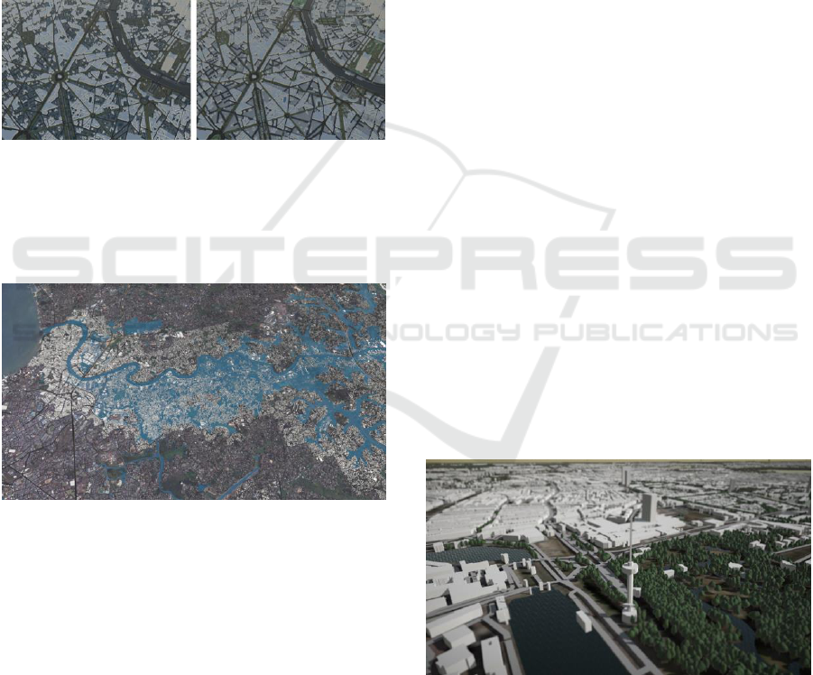
Alternatively an aerial map can serve as a base

layer by providing a Web Mapping Service (WMS)

for such tiles (Figure 4). This creates a better

understanding of the terrain type and land cover. But

it comes with the risk of being low in resolution or

having colour differences between tiles due to

different times of photography or cloud cover.

Figure 4: Difference between an aerial WMS layer and tile

generated with Maperitive.

Additionally, georeferenced shapefiles can be

loaded on top of the created geometry to visualise

different kinds of data (Figure 5).

Figure 5: City of Colombo, Sri Lanka with the May 2016

flood extend map added (data courtesy of Survey

Department of Sri Lanka).

4.1.2 Mesh Colliders

The default “mesh colliders” of Unity are used to

build a collision mesh for the generated terrain tiles.

These can be used to perform hit detection using ray

casting techniques. Raycasts are used to position

certain objects (trees, roads) exactly on the terrain,

such that they do not float above the terrain.

All LOD levels share the collider of the highest

and most accurate LOD level. This could lead to

some floating objects on the terrain, but only when

these object are so far away from the camera that

such errors are practically invisible. When the user

gets closer to the terrain objects, the terrain will be

shown in the highest LOD level and therefore

objects should match with the terrain.

4.2 Building Generation

The building data that OSM contains is most of the

time a “floor plan”. So only the vertices are provided

that composes the outline of the building.

Before buildings are generated, some pre-

processing scripts using the GDAL libraries

(Gdal.org, 2016) are used to clip the buildings that

belong to a certain tile. The tile’s x-y coordinates are

stored for each row in the database to make it easy to

query.

Buildings are generated for each tile rather than

as one big mesh. The latter would make it

impossible to load data dynamically depending on

the camera frustum position. Currently these tiles are

not loaded on demand yet, which is a feature that is

planned for the future. Using tiles the rendering can

also effectively cull buildings that are not visible to

the camera. If it were just multiple large meshes

covering the whole terrain area, one building could

trigger the rendering of thousands of other buildings,

therefore increasing the number of rendered

triangles.

Some buildings have additional information such

as height (height of the building), number of floors

and minimum height (distance from the ground). A

single building can be made of several parts. In this

case the OSM attribute building:part will be set to

“yes”. Combined with the attribute min_height, this

is a powerful option to create buildings which are

more than just an extruded floor plan, as building

parts can be stacked on top of each other (Figure 6).

Figure 6: Euromast tower in Rotterdam, the Netherlands.

It consists of multiple geometry elements using the

“building:part=yes” tag.

If the height of the building is available, this

information is used directly in order to extrude the

mesh. Otherwise, when the number of floors is

IVAPP 2017 - International Conference on Information Visualization Theory and Applications

254

known, the “formula for calculating the height of a

‘mixed-use’ or ‘function unknown’ tall building”

(Ctbuh.org, 2016) is used to determine building

height. When none of these are available, a default

height of 6 meters is used.

To generate 3D buildings several steps need to

be performed. The building information is already

stored per OSM tile in an earlier step. To make

culling of buildings straightforward, all buildings are

attached to the tile on which they are standing. For

each tile we execute the following steps:

Query SQLiteDB for buildings of tile

For each building in tile

Merge adjacent vertices to remove

building walls

Tessellate outline to triangles

Copy outline and elevate by building

height to create ceiling

Build walls between floor and

ceiling

Boundary information is returned by the tessellation

library, which we use to build the “roof” of the 3D

building. This is a copy of all floor plan vertices

where the y component has been increased by either

the calculated height or a fixed default height value.

Then we generate the walls by looping through

the edges of the buildings and generating triangles

for each inner or outer edge.

All these generated vertices are added to the

meshbuilder class which will automatically build

meshes taking into account Unity’s maximum vertex

limit of 2

^16

(65536) vertices into account.

Each building has a white diffuse colour. OSM

data sometimes contains wall colour information but

this is not so common. Therefore it was decided to

proceed with a uniform colour approach, while

skipping efforts to texture buildings with a collection

of premade wall textures.

4.2.1 Fixed Model Buildings

A number of buildings are not dynamically

generated. Often buildings or structures are

described by a point object (feature) instead of a

polygon and therefore do not have the necessary

information to generate a 3D model.

In this case some prebuilt meshes are used. For

example, for objects such as: high voltage towers,

windmills and wind turbines. Occasionally more

information is available for an object: the type of

high voltage tower (Tag:power=tower, -

OpenStreetMap Wiki, 2016) or the blade diameter of

a wind turbine (Tag:generator:source=wind -

OpenStreetMap Wiki, 2016). With this information,

it is possible to select a 3D mesh from a library of

prebuilt 3D meshes. Currently in this project only

one pre-made mesh is used per recognized point

object.

4.3 Trees and Forested Areas

Tree placement in this application takes three types

of OSM data sources into account. The land use type

landuse=forest is used for random tree placement

while sometimes an actual single tree is defined

(natural=tree) or a row of trees (natural=tree_row).

4.3.1 Forest Areas

The land use type forest is used to randomly place

trees in a specified area. No trees should be

generated outside these areas. Therefore a tree

placing algorithm has been implemented. Polygons

in this algorithm are created using the

LibTessDotNet library which also takes care of

holes in the geometry.

For each polygon of natural type forest

Tessellate to a 2D mesh using the

polygon outline

Calculate expected tree count

Begin loop for expected tree count

Choose random triangle of polygon

Get random point in selected

triangle by using barycentric

coordinates

Determine if there is already a

tree at the given random location

using a radius test

If no tree nearby

Place tree and continue

Else

Try another random location up

to three times.

If no acceptable location is

found, skip tree and continue.

The maximum number of trees that are placed

per polygon is calculated using the area of a polygon

multiplied with a tree density factor. A density of 1.0

means that there will be one tree per square unit of

the polygon. An absolute maximum regardless of

polygon size ensures that very large polygons will

not generate thousands of trees.

Open Data Sources for 3D Data Visualisation - Generating 3D Worlds based on OpenStreetMaps Data

255

4.3.2 Reducing Uniformity of Trees

The vertices of trees are modified by a randomiser

function to give each tree more of an individual and

unique look (Figure 7). First, the size is uniformly

modified using a scale of 0.9 – 1.1 times the actual

size. Therefore, all the trees vary in size. Secondly,

the rotation of the tree is changed. Rotation of the x-

axis is from 0 to 360 degrees and on the y- and z-

axis the angle is between -2 and 2 degrees to make

sure that trees are not all pointing upwards and

perfectly straight. Finally, all trees have some colour

variation applied by using vertex colours. For each

tree a random greyscale colour is determined

(between RGB 100 to 255), which is then applied to

all the tree vertices. The trees are then added to the

meshbuilder class which will again make sure that

meshes are split when reaching Unity’s mesh limit,

similar to the construction of buildings. The trees

object will become a child of the terrain tile in order

to perform efficient frustum culling. When the tile

becomes invisible to the camera, so will all the trees

on top of it.

Figure 7: Trees without variation (left) and with (right).

When rendering, the fragment shader will multiply

the tree’s texture colour with the vertex colour,

giving each tree a different colour. All these steps

combined lead to a tree placement system which

creates diverse forests, while keeping the rendering

batches intact. This means that there is no

performance loss for having many randomised trees

compared to non-randomised trees.

4.3.3 Level of Detail for Trees

Unity’s own LOD system is used to reduce the

number of triangles rendered for trees that are far

away. A LOD system tries to lower the number of

rendered triangles by replacing detailed meshes with

meshes that have a lower polygon count. These

systems work, using the fact that in perspective

views, objects become smaller when distance to the

camera is increased. With properly setup LOD

levels, it is unlikely for the user to notice the

changing geometry.

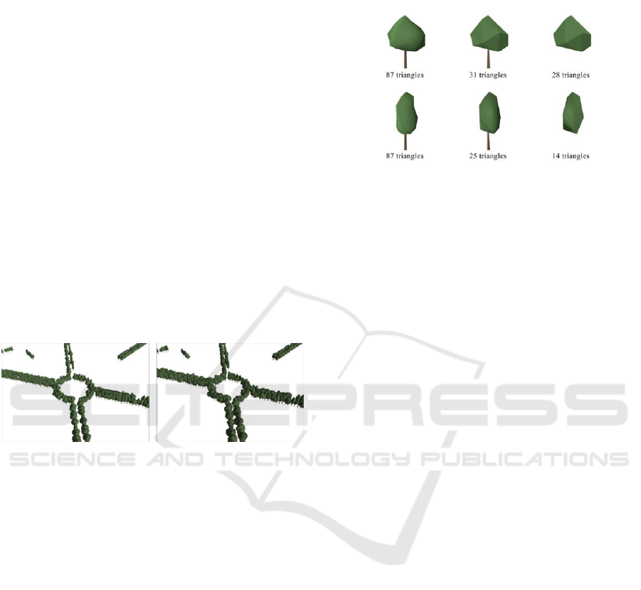
For each tree type, three different meshes have

been created in 3D modelling software: A normal

“base” tree and two types of low-polygon meshes

based upon the base tree (Figure 8).

Figure 8: Two types of trees and their three LOD levels.

The simplified trees are made like this to prevent

“popping” of the geometry. Three meshbuilder

classes are used simultaneously to generate the LOD

meshes. Each tree that is placed inside the first LOD

(high detail) meshbuilder is also automatically added

to the other two mesh builders. This will

immediately create the meshes for the medium and

low-polygon trees. Unity’s LODGroup component is

then added to this object so that Unity can

automatically determine when to render which mesh

at what distance.

4.4 Infrastructure

Various types of infrastructure are visualised as

well: Most types of car roads and railways are

visualised. The 3D models of the roads are generated

using the linestrings that are available from the OSM

data. OSM provides many categories for these. The

data is specifically filtered as follows: ‘unclassified’,

‘motorway_link’, ‘road’, ‘motorway’, ‘trunk_link’,

‘primary_link’, ‘service’, ’secondary_link’,

‘tertiary_link’, ’primary’, ’secondary’, ‘tertiary’

and ’residential’. Some categories are currently

skipped (e.g. trails) because they are rather small

and do not add significant detail to the virtual world.

They might be visible on the ground layer tiles.

An important aspect of roads that requires

attention is multiple layered roads such as

intersections, tunnels and bridges. OSM data has a

solution for objects which share the same x-y

coordinates but not elevation. The attribute layer

makes it possible to distinguish these. This way 3D

roads can be constructed which are layered on top of

each other or join two different levels together, such

as intersection junctions.

The default width of the roads is 5 meters.

Additionally, width is calculated when properties are

available such as the number of lanes or if an actual

IVAPP 2017 - International Conference on Information Visualization Theory and Applications

256

width has been set. The width of a single lane is

currently configured to be 3.5 meters. This number

varies internationally, however. The road meshes are

generated by using a quadratic Bézier curve

algorithm. Corners become rather angular when road

sections are drawn straight from point to point.

These quadratic curves provide much smoother and

more realistic representation of the roads (Figure 9).

Figure 9: Top-down view of point to point roads (left) and

quadratic curves (right).

4.5 Water Surfaces

Various sources of water surfaces can be found in

OSM data; these are of the type multipolygon in the

earlier generated SQLite database. OSM data has

many classifications of water types (e.g. rivers,

lakes, canals, etc.). These polygons are tessellated

directly without additional processing. One aspect

that has to be considered is that some water surfaces

such as oceans might not be mapped in OSM as

polygons. Rather, their coastlines have been

mapped. Datasets which contain these as polygons

can be downloaded freely (Openstreetmapdata.com,

2016). Texture mapping of these water surfaces is

based upon their absolute position in the virtual

world. A variation of flow maps (Vlachos, 2010)

gives these surfaces more water-like dynamics.

Normal implementations of the flow maps

commonly use textures for velocities of the water.

But in our water surfaces vertex colours are used

instead, as there is no need for high resolution

flowing water, while also reducing the memory

footprint for each surface. In order to make sure

there are no unexpected colour changes in the water,

the polygons do not share their vertices and every

triangle has unique vertices.

5 CONCLUSIONS AND FUTURE

WORK

This paper covered an approach to generate a 3D

virtual world based upon OSM data (Figure 10).

Various approaches have been shown that were used

to generate terrain tiles, perform tree placement,

create infrastructure of roads and railways, plus

generating polygons of water surfaces.

There is still room for improvement by

implementing various other techniques for

generating efficient geometry. Recent versions of

Unity support GPU instancing. This creates

opportunities in displaying massive amounts of

geometry, such as trees, without having an enormous

performance impact. Recent DirectX versions

support dynamic tessellation which allows the

creation of details on the vertex shader itself without

having to generate additional vertices on the CPU

side.

Another improvement would be to generate

geometry on the fly instead of only once during start

up. Dynamic creation of tiles makes it possible to

explore any place in the world without running into

potential memory issues, as well as reducing loading

times at the start of the virtual environment.

Batching of terrain tiles could be further

optimized by making use of texture atlases. A single

4096x4096 pixels texture can fit up to 16x16 terrain

textures. This would reduce the number of draw

calls by a factor of 256. Care needs to be taken

regarding the mip-mapping of these texture atlases

as border pixels might bleed to the texture of

neighbouring tiles. It is very likely that some of the

pre-processing can be skipped by making use of the

OSM Spatialite-tools (Gaia-gis.it, 2016). These tools

create a SQLite database with spatial extensions

which provide a fast way to query geometry from

the database. As well as keeping OSM node

references, which potentially allows better merging

of geometry.

Figure 10: Visualisation of Hamburg, Germany.

ACKNOWLEDGEMENTS

This research is part of the Strategic Research

Programme on Software Innovation of Deltares,

Open Data Sources for 3D Data Visualisation - Generating 3D Worlds based on OpenStreetMaps Data

257

funded by the Ministry of Economic Affairs, the

Netherlands.

REFERENCES

Actionstreetmap.github.io. (2016). ActionStreetMap.

Available at: https://actionstreetmap.github.io/demo/

(Accessed 17 Oct. 2016).

BinomialLLC/crunch. (2016). BinomialLLC/crunch.

Available at: https://github.com/BinomialLLC/crunch

(Accessed 17 Oct. 2016).

Ctbuh.org. (2016). Calculating the height of a tall building

where only the number of stories is known. Available

at:http://www.ctbuh.org/HighRiseInfo/TallestDatabase

/Criteria/HeightCalculator/tabid/1007/language/en-

GB/Default.aspx (Accessed 17 Oct. 2016).

Download.geofabrik.de. (2016). Download.geofabrik.de.

Available at: http://download.geofabrik.de (Accessed

17 Oct. 2016).

F4map Demo - Interactive 3D map. (2016). F4map Demo

- Interactive 3D map. Available at:

http://demo.f4map.com/ (Accessed 18 Oct. 2016).

Garmin.openstreetmap.nl. (2016). Free worldwide Garmin

maps from OpenStreetMap. Available at:

http://garmin.openstreetmap.nl/ (Accessed 17 Oct.

2016).

Garland, M. and Heckbert, P. (1995). Fast Polygonal

Approximation of Terrains and Height Fields.

Gdal.org. (2016). GDAL: ogr2ogr. Available at:

http://www.gdal.org/ogr2ogr.html (Accessed 17 Oct.

2016).

Hotosm.org. (2016). Projects | Humanitarian

OpenStreetMap Team. Available at:

https://hotosm.org/projects (Accessed 17 Oct. 2016).

Kärkkäinen, S. (2016). Tactile Maps Easily | Touch

Mapper. Touch Mapper - Tactile Maps for the

Visually Impaired. Available at: https://touch-

mapper.org (Accessed 17 Oct. 2016).

Knerr, T. (2016). OSM2World. Osm2world.org. Available

at: http://osm2world.org/ (Accessed 17 Oct. 2016).

OpenStreetMap. (2016). OpenStreetMap. Available at:

http://www.openstreetmap.org/about (Accessed 17

Oct. 2016).

Openstreetmapdata.com. (2016). Coastline datasets | Data

| OpenStreetMapData. Available at: http://openstreet

mapdata.com/data/coast (Accessed 17 Oct. 2016).

Osmbuildings.github.io. (2016). OSMBuildings Index.

Available at: http://osmbuildings.github.io/

OSMBuildings/ (Accessed 17 Oct. 2016).

Osmfilter - OpenStreetMap Wiki. (2016). Osmfilter -

OpenStreetMap Wiki. Available at:

http://wiki.openstreetmap.org/wiki/Osmfilter

(Accessed 17 Oct. 2016).

Osmand.net. (2016). OsmAnd - Offline Mobile Maps and

Navigation. Available at: http://osmand.net/features

(Accessed 17 Oct. 2016).

Maperitive.net. (2016). Maperitive. Available at:

http://maperitive.net/ (Accessed 18 Oct. 2016).

Shuttle Radar Topography Mission. (2016). Shuttle Radar

Topography Mission. Available at:

http://www2.jpl.nasa.gov/srtm/ (Accessed 18 Oct.

2016).

Gaia-gis.it. (2016). spatialite-tools: spatialite-tools.

Available at: https://www.gaia-gis.it/fossil/spatialite-

tools/index (Accessed 20 Oct. 2016).

speps/LibTessDotNet. (2016). speps/LibTessDotNet.

Available at: https://github.com/speps/LibTessDotNet

(Accessed 17 Oct. 2016).

Stats - OpenStreetMap Wiki. (2016). Stats -

OpenStreetMap Wiki. Available at:

http://wiki.openstreetmap.org/wiki/Stats (Accessed 17

Oct. 2016).

Tag:generator:source=wind - OpenStreetMap Wiki.

(2016). Tag:generator:source=wind - OpenStreetMap

Wiki. Available at: http://wiki.openstreetmap.org/

wiki/Tag:generator:source%3Dwind (Accessed 17

Oct. 2016).

Tag:power=tower. (2016). Tag:power=tower -

OpenStreetMap Wiki. Available at: http://wiki.open

streetmap.org/wiki/Tag:power%3Dtower (Accessed

17 Oct. 2016).

Triangle.NET. (2016). Triangle.NET. Available at:

https://triangle.codeplex.com/ (Accessed 17 Oct.

2016).

Unity. (2016). Unity - Game Engine. (online) Available at:

https://unity3d.com/ (Accessed 20 Oct. 2016].

UDST/vizicities. (2016). UDST/vizicities. Available at:

https://github.com/UDST/vizicities (Accessed 17 Oct.

2016).

Paologianfrancesco.com. (2016). urban shape - paolo

gianfrancesco. Available at: http://www.paolo

gianfrancesco.com/graphic/urban-shape (Accessed 17

Oct. 2016).

Vlachos, A. (2010). Water Flow in Portal 2. Slides at:

http://www.valvesoftware.com/publications/2010/sigg

raph2010_vlachos_waterflow.pdf (Accessed 17 Oct.

2016).

Zoom levels - OpenStreetMap Wiki. (2016). Zoom levels -

OpenStreetMap Wiki. Available at: http://wiki.

openstreetmap.org/wiki/Zoom_levels (Accessed 17

Oct. 2016).

Xapi - OpenStreetMap Wiki. (2016). Xapi -

OpenStreetMap Wiki. Available at:

http://wiki.openstreetmap.org/wiki/Xapi (Accessed 17

Oct. 2016).

IVAPP 2017 - International Conference on Information Visualization Theory and Applications

258