
Research on Seamless Image Stitching based on Depth Map
Chengming Zou, Pei Wu and Zeqian Xu
School of Computer Science and Technology, Wuhan University of Technology, Luoshi Road, Wuhan, China
{zoucm, wupei-pei}@whut.edu.cn, 937790017@qq.com
Keywords: Image Extraction, Image Stitching, Collaborative Calibration, Multi-band Blending.
Abstract: Considering the slow speed of panorama image stitching and the ghosting of traditional image stitching
algorithms, we propose a solution by improving the classical image stitching algorithm. Firstly, a SIFT
algorithm based on block matching is used for feature matching which was proposed in our previously
published paper. Then, the collaborative stitching of the color and depth cameras is applied to further enhance
the accuracy of image matching. Finally, according to a multi-band blending algorithm, we obtain a panoramic
image of high quality through image fusion. The proposed algorithm is based on two problems in the
technology of feature-based image stitching algorithm, the algorithm’s real-time and ghosting. A series of
experiments show that the accuracy and reliability of the improved algorithm have been increased. Besides a
comparison with AutoStitch algorithm illustrates the advantage of the improved algorithm in efficiency and
quality of stitching.
1 INTRODUCTION
Currently image stitching technology have achieved
rapid development in many fields such as weather
forecasting, space exploration, super resolution
processing, reconstruction, military reconnaissance
and digital cameras. The task of seamless image is to
obtain a pair of high resolution panoramic images
which are of big vision and no seam by processing a
group of image sequence that have an overlapping
area (Brown 1999).
A number of rsearchers have deeply studied about
it. In the 1990s, Richard Szeliski (1996) proposed a
mosaic model according to the camera’s motion,
which was processed by the iterative nonlinear
minimization operator (Levenberg Marquardt, LM)
to complete the image stitching. Based on the
frequency domain characteristic of the image, two
dimensional Fourier transform is used to solve the
geometry transformation between different images
and thus image mosaic is achieved. Jang(1999)
implemented a panorama stitching algorithm based
on equal match, the source image of which is
photographed by rotating in the horizontal direction,
so it doesn’t apply in general situation. In 2003,
Brown and Lowe proposed an image mosaic
algorithm based on SIFT feature extraction, which
had a huge impact in the field of image stitching. The
algorithm is robust, and can automatically identify a
plurality of view sand reject noise in the image. But
its’ camera model is so simple that it often affected by
parallax and results in obvious ghosting. Wherein,
SIFT algorithm was proposed in 1999 by them and
further improved in 2004. The feature points acquired
by SIFT operator are of scale and rotational invariant,
which makes SIFT algorithm be widely used. In
2003, Mikolajczyk and Smith proposed an intelligent
stitching algorithm on the basis of Szeliski’s (2000)
panoramic image stitching model. The algorithm can
select a proper splicing model according to the
camera’s movement, which optimizes the efficiency
and quality of image stitching. One year later, after
more deep research, they improved the algorithm to
intelligently select the best stitching model, which
greatly enhanced the automation of the algorithm.
Since then, adaptive issue has become a hot in the
field of image stitching (Gholipour 2007, Brown and
Lowe 2007). Brown and Lowe, who did further
research to their previous work, implemented a
panoramic image stitching image which can
automatically stitch disorder images
10
. The algorithm
used a probabilistic model to choose the images
associated with the panoramic image from the
disorder image sequence, thereby removing noise in
the image and realizing panoramic stitching. In the
early 10 years of the 21th century, J. Shin (2010)
presented a new method of stitching binding the
energy spectrum technology, which committed to
Zou, C., Wu, P. and Xu, Z.
Research on Seamless Image Stitching based on Depth Map.
DOI: 10.5220/0006146303410350
In Proceedings of the 6th International Conference on Pattern Recognition Applications and Methods (ICPRAM 2017), pages 341-350
ISBN: 978-989-758-222-6
Copyright
c
2017 by SCITEPRESS – Science and Technology Publications, Lda. All rights reserved
341

Algorithm 1: Seamless Mosaic Based on Depth map.
addressing the problem of ghosting. This algorithm
achieved relatively good results but sacrificed in
actual effect on a certain degree. Another important
step in the process of image stitching, image fusion
has huge influence to the quality of image
stitching. The common mean of fusion is to fuse
overlapping areas with weighted splicing operator,
the main two methods of which are the cap-like
function weighted approach and fade out and in
weighted method (Gao 2011). The principle of the
cap-like function is to spread to the surrounding
pixels from the center of the overlapping area and
make the weight descend (Singh 2007).
Through detailed research work, we found that the
traditional stitching algorithms based on feature
matching are robust, and they can successfully get the
final mosaic images. However, there are two
commonly problems. First, the speed of panorama
image stitching is slow. Because the image stitching
algorithms need to extract feature points towards all
the images in the image sets, which will take a long
time. Second, in the actual shooting process, there
will be disparity which will increase the difficulty of
image registration and cause significant ghosting.
Considering above two issues, we propose a
solution by improving the classical image stitching
algorithm. Firstly, a SIFT algorithm based on block
matching is used for feature matching which was
proposed in our previously published paper and
proved to be robust(Zou 2015). And the detailed
description can refer to reference 15. Then, the
collaborative stitching of the color and depth cameras
is applied to further enhance the accuracy of image
matching. Finally, according to a multi-band blending
algorithm, we obtain a panoramic image of high
quality through image fusion. And the specific
process of image stitching algorithm based on depth
image is shown as algorithm1.
The proposed algorithm is based on two problems
in the technology of feature-based image stitching
algorithm, the algorithm’s real-time and ghosting. A
series of experiments show that the accuracy and
reliability of the improved algorithm have been
increased. Besides a comparison with AutoStitch
algorithm illustrates the advantage of the improved
algorithm in efficiency and quality of stitching.
2 COLLABORATIVE
CALIBRATION BETWEEN THE
DEPTHC CAMERA AND
COLOR CAMERA
In Brown’s and Lowe’s experiment, they used a
simple camera model, pinhole camera model, which
didn't take some factors into consideration such as the
geometric distortion of camera, the jitter and skew
while screening. The parameters they used to describe
the camera were so easy, so it may cause very serious
ghosting. To solve this problem, we use a
collaborative calibration between the color and depth
cameras to align the depth camera to the color camera.
After determining the internal and external
parameters of those cameras, we can get the
projection transformation matrix. The system uses a
flat calibration method, and the steps are as follows.
ICPRAM 2017 - 6th International Conference on Pattern Recognition Applications and Methods
342
2.1 Calibration
Depth camera can increase a channel to obtain the
scene information for the computer. It is possible to
build up the real-time three-dimensional scene
through the real-time depth data of depth camera.
However, in order to reconstruct a three-dimensional
coordinate through the measured data of camera, the
data in depth picture must to be aligned to the color
pixels. And the process of alignment depends on the
results of camera calibration. Because we can obtain
the parameters through camera calibration which are
necessary for alignment. Calibration includes the
respective internal parameters and the external
parameters between color and depth cameras. Color
camera has been extensively studied. For depth
camera, the existing research cannot meet the balance
of accuracy and speed. And the results are easy to be
influenced by the noise of depth data. In this case,
we studied the joint calibration of color and depth
cameras.
(a) (b)
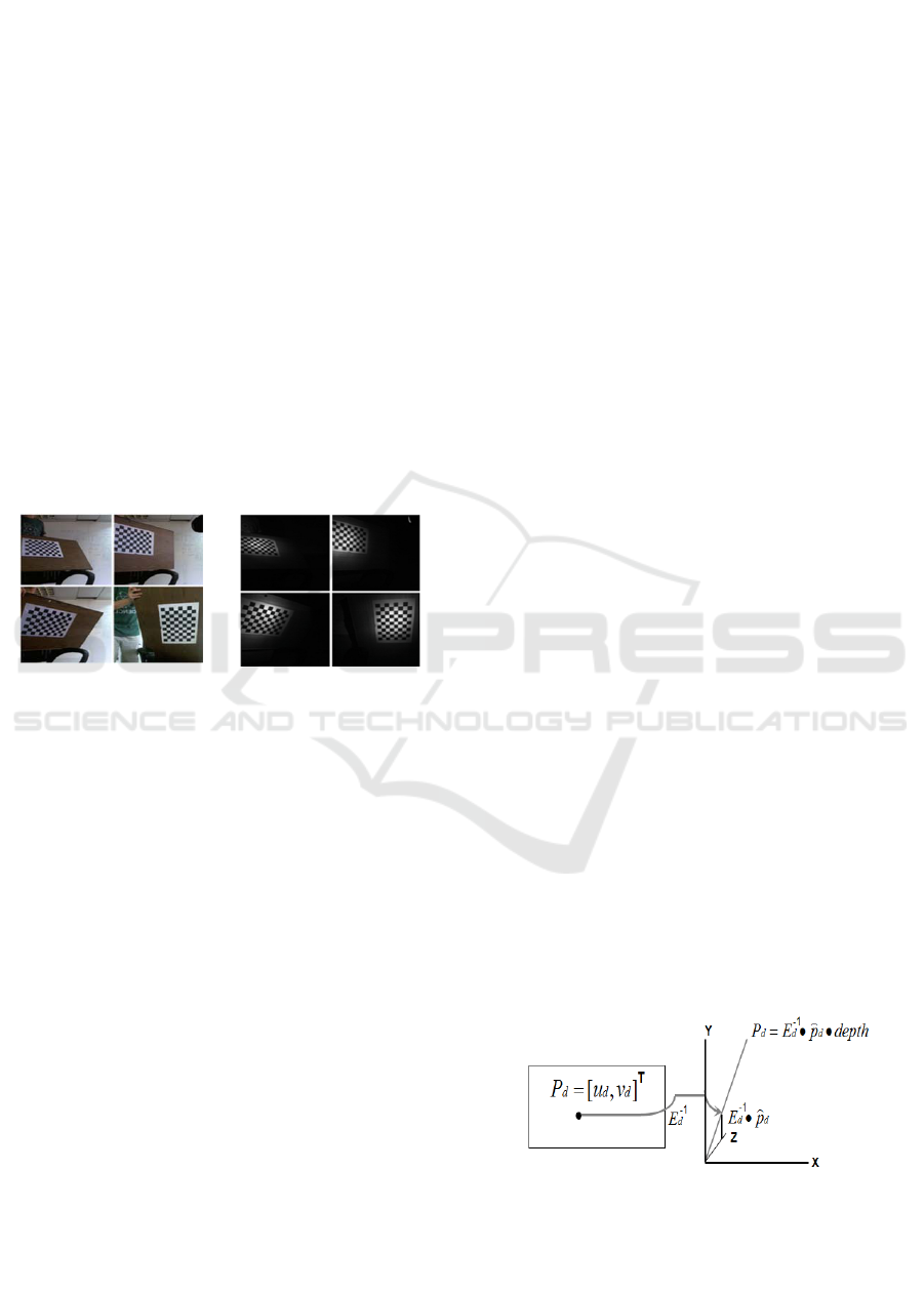
Figure 1: Calibration of camera: (a) color camera and (b)
depth camera.
To achieve the joint calibration of the color and
depth cameras, we take the pictures of the
checkerboard at different perspectives with the
cameras to be calibrated, and calculate the matrix of
the inner parameters of the camera and its outer
parameters related to each image with the camera
calibration interface provided by OpenCv library.
Kinect depth camera uses an infrared speckle
transmitter to emit infrared beam. Then when the light
beam irradiates to the surface and reflects back to the
depth camera, the depth camera will calculate the
depth of the object through the geometric relationship
between returning bulk spots. Figure 1 shows the
calibration images of color camera and depth camera.
And the right picture is the infrared figure
corresponding to the color image. We can
respectively calculate the internal parameters of the
depth camera and color camera from Fig.1. Here, we
use the interface provided by OpenCv to obtain the
camera parameters. The distortion parameters of the
color camera is [0.025163 -0.118850-0.006536-
0.001345] and that of the depth camera is [-0.094718
0.284224 -0.005630-0.001429]. Then the internal
parameters of the color camera and depth camera are:
E
=
554.952628 0.000000 327.545377
0.000000 555.959694 248.218614
0.000000 0.000000 1.000000
=
597.599759 0.000000 322.978715
0.000000 597.651554 239.635289
0.000000 0.000000 1.000000
There are few points to be noted during the
calibration. First, the calibration board should be as
large as possible, at least to reach the size of A3 paper.
Second, the angle between the board plane and the
camera bead plane can’t be too large, which should
be controlled below 45 degrees. Third, the tilts and
positions of the board need to be as diverse as
possible, because those boards parallel to each other
have no help to the calibration results. Fourth, there
should be at least ten images used to calibrate, which
can help to improve the accuracy. Fifth, the resolution
of the camera should be properly set, and the aspect
ratio is preferably the same as the depth map.
2.2 Projection Transformation Matrix
After the calibration of color camera, we need to
obtain the projection transformation matrix, depth
camera’s internal parameters and outside parameters
related to color camera.
In our calibration system, color camera is fixed on
depth camera and they remain parallel. So we only
need to do some certain translation transformation
to project the depth data into the coordinate system of
color camera. Then we need project the depth data
into color image to form the final depth buffer.
During the process, we must note that due to the
different resolution of those two cameras, the depth
buffer data and color data cannot be fully
realized alignment in the strict sense, but we
only need part of the depth data to verify, therefore,
depth image need not be enhanced.
Figure 2: The transformation from depth data to 3D
coordinates.
On the corresponding area of the depth
checkerboard image, we randomly calibrate a block
Research on Seamless Image Stitching based on Depth Map
343
regardless of the shape of it, but we must ensure that
the number of pixel points is greater than ten. As
Figure 2, for a pixel point on the block, α represents
its disparity. And depth is got from (1), through which
the back projection is achieved and converted to the 3
dimensional coordinate system to get the final 3D
point
(
=
∙̂
∙ℎ).And ̂
(̂
=
[
,
,1]
) is the homogeneous coordinate of
.
After restoring the 3D coordinates for all the pixel
points through their depth information, we can get the
3D point cloud.
ℎ
=−
0.075
tan
(
0.0002157−0.2356
)
[]
(1)
Then we need to calculate the projection
matrix
. While converting its pixel point
to
the color camera’s coordinate, it can be expressed
as
′
(
p
′
=
∙p
). While the checkerboard is
fit on the plate, the checkerboard acquired by color
camera is on the same plane as that acquired by depth
camera. That’s to say that
′
falls on the plane ofthe
checkerboard acquired by color camera, so p
′
is fit
to (2). Eliminating irrelevant variables, we can get
equation as (3). For the point j in the sample i, we can
get the equation as (4).
is the plot of the ̂
of
point
j
in sample
i
and depth, and the vector can be
calculated based on the sample. Besides =
∙
represents the plot of the rotation matrix
and translate vector matrix and the inverse of internal
parameters matrix of depth camera.
∙
′
=
(2)
∙
∙
∙
̂
∙ℎ+
∙
=
(3)
∙∙
+
∙
=
(4)
The process of establishing and solving equations
is as follows:
H=
h
h
h
h
h
h
h
h
h
=[
,
,
]
=[
,
,
]
=[
′
,
′
,
′
]
=
=
Then
is represented as (5) (
=
).
And
=b
is commonly replaced by (6). For M
times’ experiments with
points in each
experiment, we can get (7). In this equation,
represents the weight from this point to the equations.
Through the least squares method we can get the
value of
X
, and then get the value of Hand
.
=[x
r
′
,
y
r
′
,z
r
′
,x
r
′
,
y
r
′
,y
r
′
,z
r
′
,
x
r
′
,
y
r
′
,z
r
′
,r
′
,r
′
,r
′
]
(5)
=
(6)
∙
∙
∙
=
∙
∙
(7)
Next we need to remove two types of noise, the
one of which is generated by the change of the
distance from depth camera to the object, while
another of which is generated by the depth camera
when acquiring depth images. Here we use the weight
coefficienta
=φ
∗∅
to remove them.
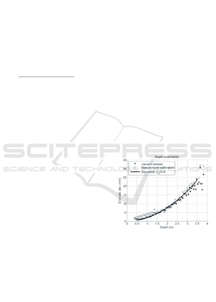
Figure 3: Solution of homography.
Kinect depth camera will produce noise along
with the change of depth due to the principle of itself.
Figure 3 shows the relationship between noise and
depth, from which we can find that noise is
proportional to the value of depth. So for t he depth
data in different areas, we need to add different
penalty coefficient, which is shown as (8).
ICPRAM 2017 - 6th International Conference on Pattern Recognition Applications and Methods
344
=
1
1+
1.2−ℎ
0.6
ℎ<1.2
11.2≤ℎ≤3.5
1
1+
ℎ−3.5
1.5
ℎ>3.5
(8)
Through above steps, we have got the depth point
cloud of the data of group i. Assuming that the
equations of the plane is as n
∙X=δ
.
n
represents the normal vector of the flat plane, and
δ
represents vertical distance from t-he origin of
camera coordinate to the flat. Suppose P
is a point on
flat. Because we have got the internal parameters
matrix of kinect depth camera,P
=E
∙p
′
. p
′
=
p
∙depth represents the product of the depth and
the 2D homogeneous coordinates of the pixel point
on t-he area calibrated manually.n
,
=E
∙n, son
,
∙
p
′
=δ. According top
′
, using Least Squares me-
thod to get n
′
. For the point p
′
on the area
calibrated manually, φ
can be defined as (9).
=
0
,
∙
′
−
>0.015∙
1
,
∙
′
−
≤0.015∙
(9)
2.3 Homograph
Those associated images which are of overlapping
area will be the source image of the panorama
stitching. Because we have got the related blocks
between the images, the matching relationship can be
easily obtained with the related blocks. During the
process of feature matching, we have got many
matching relationship of feature points. Then, to
achieve image stitch, we need obtain the homography
matrix between stitching images by using the result
of camera calibration, the internal control matrix of
camera and the out parameters in relation to each
image.
Homography refers to a reversible transformation
from the real projective plane to the photography
plane (Umeyama 1991, Chen 1994). In the domain of
computer vision, any two images in the same space
can be associated through homography (Triggs 2000).
We use the interface of OpenCV to solve the
homography matrix, the principle of which is as
follows. It calculates the rotation matrix and
translation vector of each field of view by using the
various images of a same project at different viewing
angles. The rotation matrix and translation vector
totally have six parameters, and the internal
parameter matrix of the camera has four parameters.
So, for each field of view, there are 6 non-constant
parameters and 4 constant parameters needed to be
solved. Mapping a square to a quadrilateral can be
described with 4 two-dimensional points. Suppose
that the vertex coordinates of the square on the
physical plane is (u,v) and the coordinates of the
related points on the imager is (x, y), the relationship
between them can be described as (10) and (11). After
substituting the coordinates of the four points into the
above formulas in turn, we can get 8 equations. That’s
to say that a field of view of flat checkerboard can
provide 8 equations. Therefore, it needs 2 fields of
view (two images) to solve above 10 parameters.
Besides, the points on the flat of original image are
connected with the points on the aim flat through the
(12) and (13). In addition, to achieve the process,
OpenCV offers an interface of C function for the
solving of homography.
(a) (b)
(c)
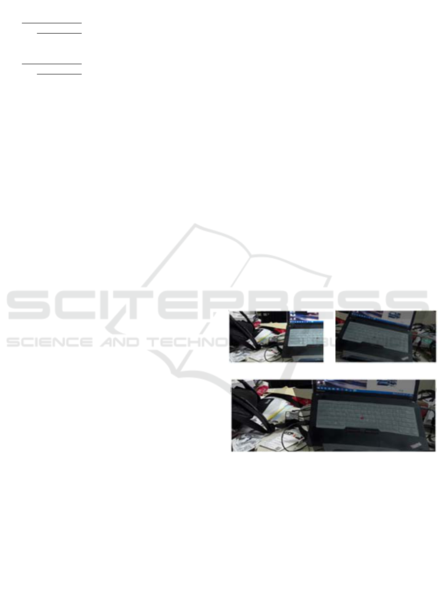
Figure 4: Solution of homography: (a) original image1, (b)
original image2 and (c) the image after registration.
Lowe used RANSAC algorithm to solve
homography, and a good result was got. Here the
RANSAC is no longer needed. We use a very small
sample to get the transformation parameters
between images, and find a solution that is best
consistent with the parameters. With this method,
we needn’t set any threshold, so the processing work
for different thresholds in different environment is
avoided and the adaptability and automation
=
(
,
)
(10)
=
(
,
)
(11)
=
,
=
(12)
=
1
,
=
1
(13)
Research on Seamless Image Stitching based on Depth Map
345

capability of the algorithm are improved. For the
color images a, b in Figure 4, we solve the
homography of these two pictures through the
external parameters of them, and implement the
registration of these two images by matrix
transformation. The result of registration is shown as
picture c in Figure 4.
3 BUNDLE ADJUSTMENT
Bundle Adjustment is used to reduce the error of
projected position transformation between the match
points of the image to be stitched (Burt 1983). The
image to be stitched is placed in a beam adjuster, and
the match image which is of the largest number
conformance will be the first to be adjusted. And in
order to place the image to the best position for
matching, the rotational transformation parameters
and focus of all the images to be stitched need be
adjusted to the same condition.
In this paper, we choose a projection error square
algorithm which is highly robust as the objective
function. Every feature point is projected into the
matched image. Besides, we will minimize the square
of the distance from it to the relative image. Given a
map u
↔u
(u
represents the position of point
k in image i), its residual is calculated using (14). p
is the map of the point related to u
from image j to
image i, the process of which is described as (15).
=
−
(14)
˜
=
˜
(15)
Error function describes the square the sum of
squared residuals generated by all images, shown as
(16). And n is the total number of images.
ℒ
(
i
)
represents the image sequence matched to image
i, and Ϝ(i,j) represents the sequence of match
feature points between i mage i and image j. We use
the error function Huber, shown as (17). This error
function mix a formal optimization strategy that L2 is
fast convergent to the domestic point (intervals less
than σ), and it has good robustness of L2 to the
peripheral points (intervals greater than σ).In the
initialization, we make the interval of peripheral point
be ∞(σ=∞), and let the pixel of σ=2in the final
strategy.
= ℎ(r
)
∈Ϝ(,)∈
ℒ
()
(16)
ℎ
(
)
=
|
|
,
|
|<
2σ
|
|
−σ
,
|
|
≥
(17)
This is a problem of non-linear least squares,
which is solved by Laffan Grignard algorithm. Every
iteration is completed with (18), in which Φis all the
parameters and r is the residuals. For the change of
parameters in covariance matrix C
, we need to
encode its prior condition. The standard difference
of angle is set to beσ
=f
̅
/10, which can help choose
a proper step size to accelerate the convergence.
=0
(18)
Image registration has utilized the parameters
obtained after camera calibration, but there are still
unknown rotation transformations in image. Since
the real camera is unlikely to be completely
level and does not tilt, if we simply assume
R=I for an image, there will be an impact on
the final output waveform panorama. Inspired by
the way of shooting panoramic images in reality, we
are able to correct the waveform influence by the
method of automatically stretching panorama. In
actual shooting, we barely twist the camera with
respect to view moment, so the camera vector X
(horizontal axis) is usually located in a plane.
Searching the zero vector of covariance matrix of the
camera vector X, we can find its normal vector u,
which is shown as (18).Because the normal vector u
of a global rotational transformation is vertical, the
waveform influence to the out-put image can be
effectively eliminated.
4 MULTI-BAND BLENDING
We choose a multi-band blending algorithm to
achieve image fusion after deep study to fusion
algorithms. On the one hand, having completed the
similar block segmentation in feature match section,
multi-band blending can make use of it further and
improve the effectiveness. On the other hand, this
algorithm has been widely used and performances
well in AutoStitch algorithm.
The core idea of multi-band fusion is based on the
view of the dam theory. Specifically, first, the image
to be stitched is divided into two parts according to its
overlapping area, so that each image is divided into
two parts which means four image blocks, where we
only use two parts. These two parts are decomposed
into different frequency bands using the Laplace
transform, which is similar to scale space. With this
ICPRAM 2017 - 6th International Conference on Pattern Recognition Applications and Methods
346
method, two Laplace pyramids are got, and then
image stitching will completed in different scales.
Finally, the final image is obtained by remodeling.
Through previous work, we have got an image
sequence like I
(x,y)(i∈{1…n}) and these
imageshave been matched. This image sequence may
be presented in a same coordinatesI
(θ,∅). To fuse
the information of different images, we set a weighted
function W
(
x,y
)
=w
(
x
)
w
(
y
)
or each image,
wherew
(
x
)
distributes as the linear change from the
center of the image to the edge of the image.
Weighting function need be re-sampled in a special
spherical coordinate system W
(x,y). A simple
image fusion method is a weighted sum along the
intensity of radiation, where the following weighting
function shown as (19) is used.
I
(
,∅
)
=
∑
I
(,∅)W
(,∅)
∑
W
(
,∅
)
(19)
I
(
θ,∅
)
is a composite spherical image by
linear mixing. However, if the stitching has a slight
error, this method may result in high frequent detail
blur. To avoid this situation, we use a multi-band
fusion algorithm proposed by Burt and Adelson
21
,
which fuses low-band image in a large scale and high-
band in a small scale. We initial the mixed weight
of the image by finding the points sequence which are
of highest confidence in image i. The process is
described by (20), in which W
(
θ,∅
)
represents
that image i is1 at the biggest weight and 0 when other
images have bigger weight. A rendered image of high
throughput ate is formed in the manner of (21) and
(22). In these equations, g
(
θ,∅
)
represents the
Gaussian function of standard deviationσ, and the
operator * denotes the convolution.
B
(
θ,∅
)
represents the spatial frequencies of the
wave length in the range ofλ∈[0,σ].We use a b-
lend weight way to fuse the different frequency bands
between images, which are shown as (23).
W
(
θ,∅
)
represents the blend weight under the
range of λ∈[0,σ]. If k ≥1, the following
Equations are got.
()
=I
−I
(
)
I
(
)
=I
∗g
W
(
)
=W
∗g
The standard deviation of Gaussian blur function
is σ
=
(2k+1)σ.This will make the later band
have the same wavelength range. For each band,
image sequences with overlapping areas are linearly
mixed, which is shown as (24). This will result in high
frequency bands are mixed in a small area, and low
frequency bands are mixed in a larger context. We
have selected a spherical coordinate systemθ,∅. In
principle, we can choose the two-
dimensional parametric surface around any view
point. And a good choice is to render to the triangle
of the sphere, and reconstruct the results of blend
weight in the surface of image sequence. This has
great advantage to processing image sequences, and
allows re-sample to another plane. But it notes that
co-ordinates θ,∅will have some distortion at the
singularities of the poles.
I
(
,∅
)
=
∑
(,∅)W
(,∅)
∑
W
(,∅)
(24)
We have conducted some experiments to compare
the multi-band image fusion algorithm with an
outdoor collection of images (as the five color source
images in Figure 5). For the limitations of kinect
camera, the experiment did not join the collaborative
stitching, which aims to illustrate the specific effects
of multi-band fusion.
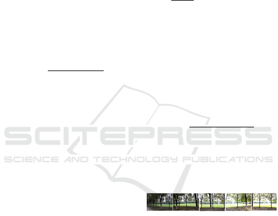
Figure 5: Color source images.
The experiment used color source images
gathered outdoors with a Huawei glory 6. The image
resolution was 3214×1840, and the size of the image
was 1.26M. These five images were captured under
different exposure and focal length whose gradients
were approximately equal to each other. Figure 6
shows the results of the fusion which did not use any
fusion method, and we can see a clear seam generated
by the different exposures of the images. While
Figure 7 shows the results of the common linear
filtering fusion, the weighted average fusion
algorithm. We can find the seam has been preliminary
eliminated, but there are a large exposure differences
between the two parts of the fused image. Because
(
,∅
)
=
1W
(
,∅
)
=arg
W
(
,∅
)
0ℎ
(20)
(
,∅
)
=I
(
,∅
)
−I
(
,∅
)
(21)
(
,∅
)
=I
(
,∅
)
∗g
(
,∅
)
(22)
(
,∅
)
=
(
,∅
)
∗g
(
,∅
)
(23)
Research on Seamless Image Stitching based on Depth Map
347
the fusion quality problems, it is difficult for this
method to deal with more complex source images.
And Figure 8 shows the results of multi-band fusion.
The seam has been fully eliminated, and the whole
image exposure is not significantly different in
different regions, so the fusion is better than the
simple weighted fusion.
Figure 6: Fusion rendering without any fusion algorithm.
Figure 7: Fusion rendering with Linear Filtering.
Figure 8: Fusion rendering with multi-band fusion
algorithm.
5 IMPLEMENTATION AND
EXPERIMENTAL RESULTS
Our experiments with different algorithms are
achieved with OpenCV library under the environment
of Intel Core i5 3210M CPU, 2.5GHZ, and 4GRAM.
This paper mainly solves the ghost due to image
registration errors and enhances the efficiency of
stitching algorithm. And we select AutoStitch
algorithm as the comparison algorithm.
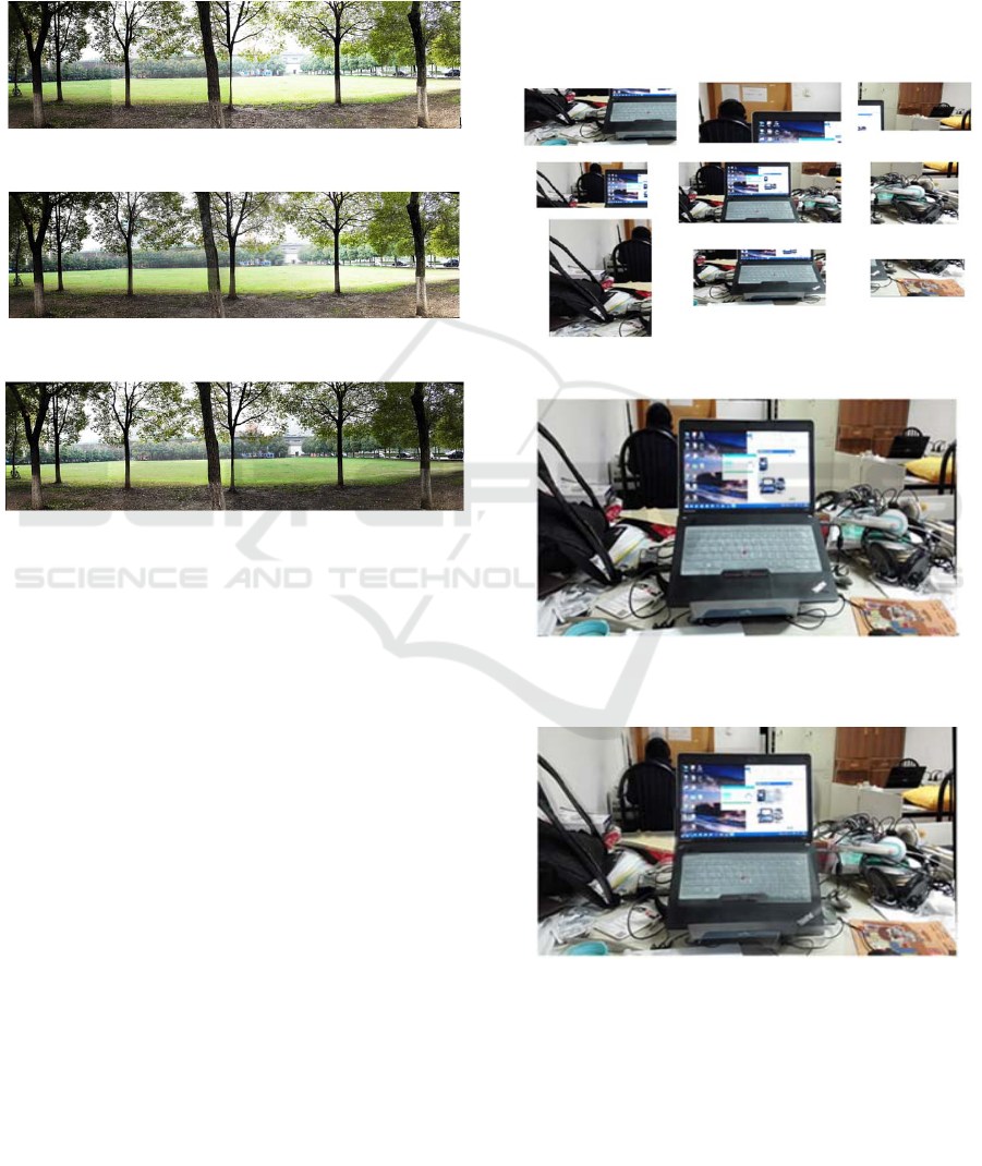
The nine experimental images are shown in
Figure 9, which are shoot with the phone (Huawei
glory6) in different positions. In order to be closer to
the real situation, the pixels of the nine source images
are adjusted to six gradients, and the aspect ratio are
roughly constant at 4:3. The pixels of the six groups
of images are 480×320, 640×480, 800×600, 1140
×850, 1520×1140 and 2100×1520. Since previous
experiments have demonstrated the overall stitching
quality of the algorithm, it is no longer to show the
corresponding depth image of each image. With the
proposed algorithm, firstly, the color images are
divided into blocks to do extract and match of feature
points with SIFT algorithm. Then, combined with the
collaborative calibration, the depth information is
attached to the color image and the final result of
image stitching is got through RANSAC algorithm
and the internal and external parameters got by
camera’s collaborative calibration. And the final
fusion image is shown as Figure 10. And Figure 11
shows the fused image by AutoStitch algorithm.
Figure 9: Experimental images gathered in lab.
Figure 10: Seamless stitching rendering with the proposed
algorithm.
Figure 11: Seamless stitching rendering with the AutoStitch
algorithm.
After a series of experiments, we select the
average value as the final experimental data. A
comparison of the time used in each stage between
the original algorithm and improved algorithm is
shown as Table 1. We can find that in the part of SIFT
ICPRAM 2017 - 6th International Conference on Pattern Recognition Applications and Methods
348

Table 1: Experimental results table.
Running
time(s)
Test 1 Test 2 Test 3
Improved
algorithm
AutoStitch Improved
algorithm
AutoStitch Improved
algorithm
AutoStitch
SIFT feature
extraction
1.68 1.85 1.86 2.03 3.17 3.45
Feature
matching
0.67 0.92 0.68 0.93 0.67 0.92
Homography
0.03 0.09 0.04 0.09 0.04 0.08
Image
stitching
and
correction
0.07 0.06 0.08 0.07 0.08 0.06
Image
fusion
1.02 1.06 1.29 1.34 1.43 1.54
Total time
3.47 3.98 3.95 4.46 4.47 5.05
Test 4 Test 5 Test 6
Improved
algorithm
AutoStitch Improved
algorithm
AutoStitch Improved
algorithm
AutoStitch
4.57 4.97 6.56 7.14 8.97 9.76
0.67 0.92 0.67 0.92 0.67 0.92
0.04 0.08 0.04 0.08 0.04 0.08
0.08 0.06 0.08 0.06 0.08 0.06
1.94 2.15 2.25 2.46 3.17 3.53
7.3 8.18 9.6 10.66 12.93 14.35
feature extraction, the SIFT algorithm based on block
matching improves approximately 8% in timeliness
compared to the AutoStitch feature extraction.
However, compared to AutoStitch algorithm, the time
consuming in feature matching of the proposed
algorithm significantly reduces. This is because that
AutoStitch builds KD tree for full image feature
points, while the improved algorithm in this paper
only builds KD tree for the feature points in
overlapping area. In the part of solving homography,
this paper uses the method of camera calibration,
while AutoStitch uses RANSAC method. As a
random sampling method, RANSAC algorithm is
poor in timeliness. In image stitching and correction
and image fusion, these two algorithms are not very
different, so the running time is almost same.
Compared to AutoStitch algorithm, the time-
consuming of improved algorithm in this paper
decreases by 10%, and we can find from Table 1 that
with the increase of image data, the reduction
percentage in time consuming of the improved
algorithm in this paper is almost unchanged. This is
because that the overlapping area is bigger with the
increase of image data, the proportion of which
remains almost unchanged in each image with respect
to the overall data.
6 CONCLUSIONS
Our research has achieved a seamless image stitching
method based on depth map. The SIFT algorithm
based on block matching effectively shield the non-
overlapping areas, which avoids the feature points
extraction and matching of the whole image and
increases the efficiency of the algorithm. The
collaborative calibration system based on the depth
camera and color camera maps the depth data into a
color image to complete registration, further
increasing the quality of image stitching.
Experiments proof that the ghosting caused by
shooting parallax and registration error significantly
Research on Seamless Image Stitching based on Depth Map
349

reduces. Combined with the actual needs, we select
the multi-band image fusion algorithm for image
fusion. Experiments to this algorithm show that the
applicability of this algorithm is great. Then, we
conduct a series of experiments and analysis to the
seamless image algorithm based on the depth image,
which increases the efficiency of stitching algorithm
and reduces the ghosting.
ACKNOWLEDGEMENTS
This research work was supported by National
Natural Science Foundation of China (NSFC) under
grant number 61503289, Science and Technology
Support Plan of Hubei Province under grant number
2015BAA120 and 2015BCE068, ESI top 1%
Disciplines Foundation in 2014 (79).
REFERENCES
Jang, K.H., 1999. Constructing Cylindrical Panoramic
Image Using Equidistant Matching. Electronics Letters,
35(20), 1715-1716.
Brown, M. & Lowe, D., 2003. Recognizing Panoramas. In
IEEE International Conference on Computer Vision.
WASHINGTON.
Lowe, D.G., 1999. Object Recognition from Local Scale-
invariant Features. In IEEE International Conference
on Computer Vision. GREECE.
Lowe, D.G., 2004. Distinctive Image Features from Scale-
Invariant Key-points. International Journal of
Computer Vision, 60(2), 91-110. Szeliski, R. & Shum,
H.Y., 2000. Creating Full View Panoramic Image
Mosaics and Environment Maps. Proc Sigraph, 251-
258.
Szeliski, R. & Shum, H.Y., 2000. Creating Full View
Panoramic Image Mosaics and Environment Maps.
Proc Sigraph, 251-258.
Mikolajczyk, k. & Schmid, C., 2003. A Performance
Evaluation of Local Descriptors. IEEE Conference on
Computer Vision & Pattern Recognition, 27(10), 257.
Gholipour, A. et al., 2007. Brain Functional Localization: a
survey of image registration techniques. IEEE
Transactions on Medical Imaging, 26(4), 427-51.
Brown, M. & Lowe, D.G., 2007. Automatic Panoramic
Image Stitching using Invariant Features. International
Journal of Computer Vision, 74(1), 59-73.
Tang, Y. & Shin, J., 2010. De-ghosting for Image Stitching
with Automatic Content-Awareness. International
Conference on Pattern Recognition, 2210-2213.
Gao, J., et al., 2011. Constructing Image Panoramas using
Dual-homography Warping. IEEE Conference on
Computer Vision & Pattern Recognition, 42(7), 49-56.
Singh, R. et al., 2007. A Mosaicing Scheme for Pose-
invariant Face Recognition. IEEE Transactions on
Systems Man & Cybernetics Society, 37(5), 1212-1225.
Zou, C.M., et al., 2015. A SIFT Algorithm Based on Block
Matching. Computer Science, 42(4), 311-315.
Umeyama, S., 1991. Least-squares Estimation of
Transformation Parameters between Two Point
Patterns. IEEE Transactions on Pattern Analysis &
Machine Intelligence, 13(4), 376-380.
Chen, Q.S., et al., 1994. Symmetric Phase-only Matched
Filtering of Fourier-Mellin Transforms for Image
Registration and Recognition. IEEE Transaction on
Pattern Analysis & Machine Intelligence, 16(12), 1156-
1168.
Triggs, B., et al., 2000. Buddle Adjustment: A Modern
Synthesis. Vision Algorithms Theory & Practice, 298-
373.
Burt, P.J., 1983. A Mutiresolution Spline with Application
to Image Mosaics. Acm Transactions on Graphics, 2(4),
217-236.
ICPRAM 2017 - 6th International Conference on Pattern Recognition Applications and Methods
350
