Multiple Target, Multiple Type Visual Tracking using a Tri-GM-PHD

Filter

Nathanael L. Baisa and Andrew Wallace

Department of Electrical, Electronic and Computer Engineering, Heriot Watt University, Edinburgh, U.K.

{nb30, a.m.wallace}@hw.ac.uk

Keywords:

Visual Tracking, Random Finite Set, Multiple Target Filtering, Gaussian Mixture, Tri-GM-PHD Filter, OSPA

Metric.

Abstract:

We propose a new framework that extends the standard Probability Hypothesis Density (PHD) ﬁlter for mul-

tiple targets having three different types, taking into account not only background false positives (clutter), but

also confusion between detections of different target types, which are in general different in character from

background clutter. Our framework extends the existing Gaussian Mixture (GM) implementation of the PHD

ﬁlter to create a tri-GM-PHD ﬁlter based on Random Finite Set (RFS) theory. The methodology is applied

to real video sequences containing three types of multiple targets in the same scene, two football teams and a

referee, using separate detections. Subsequently, Munkres’s variant of the Hungarian assignment algorithm is

used to associate tracked target identities between frames. This approach is evaluated and compared to both

raw detections and independent GM-PHD ﬁlters using the Optimal Sub-pattern Assignment (OSPA) metric

and discrimination rate. This shows the improved performance of our strategy on real video sequences.

1 INTRODUCTION

Visual detection, tracking and association of multiple

targets at each frame in a video sequence is an active

research ﬁeld. In some cases, for example for situa-

tional awareness, driver assistance and vehicle auton-

omy, there is also a necessity to distinguish between

different target types, e.g. between vehicles and more

vulnerable road users such as pedestrians and bicy-

cles to select the best sensor focus and course of ac-

tion (Matzka et al., 2012). For sports analysis we

often want to track and discriminate sub-groups of

the same target type such as the players in opposing

teams (Liu and Carr, 2014). In this and many other

examples, confusion between target types is common;

a standard histogram-based detection strategy (Dol-

lar et al., 2014) in an urban environment may provide

confused detections between pedestrians and cyclists,

and even small cars.

Traditional multi-target trackers have been based

on ﬁnding associations between targets and mea-

surements. These include Global Nearest Neigh-

bor (GNN) (Cai et al., 2006), Joint Probabilistic

Data Association Filter (JPDAF) (Rasmussen and

Hager, 2001), and Multiple Hypothesis Tracking

(MHT) (Cham and Rehg, 1999). However, these ap-

proaches have faced challenges not only in the uncer-

tainty caused by data association but also in algorith-

mic complexity that increases exponentially with the

number of targets and measurements.

To address the problem of increasing complexity,

a uniﬁed framework which directly extends single to

multiple target tracking by representing multi-target

states and observations as Random Finite Sets (RFS)

was developed by Mahler (Mahler, 2003). This es-

timates the states and cardinality of an unknown and

time varying number of targets in the scene, and al-

lows for target birth, death, clutter (false alarms), and

missing detections. Mahler (Mahler, 2003) proposed

to propagate the ﬁrst-order moment of the multi-target

posterior, called the Probability Hypothesis Density

(PHD), rather than the full multi-target posterior.

There are two popular implementations for the

PHD ﬁlter, the Gaussian Mixture (GM-PHD) (Vo and

Ma, 2006) and the Sequential Monte Carlo (SMC) or

particle-PHD ﬁlter (Vo et al., 2005). The GM-PHD

ﬁlter is used in (Zhou et al., 2014) for tracking pedes-

trians in video sequences but there is only one type of

target and the motion model is ﬁxed. As an extension,

a GM-PHD Filter was also developed in (Pasha et al.,

2009) for maneuvering targets but this employed a

Jump Markov System (JMS) that switched between

several motion models. In contrast, a particle-PHD

ﬁlter was applied in (Maggio et al., 2008) to allow for

L. Baisa N. and Wallace A.

Multiple Target, Multiple Type Visual Tracking using a Tri-GM-PHD Filter.

DOI: 10.5220/0006145704670477

In Proceedings of the 12th International Joint Conference on Computer Vision, Imaging and Computer Graphics Theory and Applications (VISIGRAPP 2017), pages 467-477

ISBN: 978-989-758-227-1

467

more complex motion models, and to cope with vari-

ation of scale, which has signiﬁcant effects not just on

object motion but also on the detection process.

Considering extensions to different target types,

Yan et al. (Wei et al., 2012) developed detection,

tracking and classiﬁcation (JDTC) of multiple tar-

gets in clutter which jointly estimates the number

of targets, their kinematic states, and types of tar-

gets (classes) from a sequence of noisy and cluttered

observation sets using a SMC-PHD ﬁlter. The dy-

namics of each target type (class) was modeled as

a class-dependent model set and the signal ampli-

tude is included in the multi-target likelihood to en-

hance the discrimination between targets from differ-

ent classes and false alarms. Similarly, a joint tar-

get tracking and classiﬁcation (JTC) algorithm was

developed in (Yang et al., 2014) using RFS which

takes into account extraneous target-originated mea-

surements (of the same type) i.e. multiple measure-

ments that originated from a target which can be mod-

eled as a Poisson RFS using linear and Gaussian as-

sumptions. In these approaches, the augmented state

vector of a target comprises the target kinematic state

and class label, i.e. the target type (class) is put into

the target state vector. However, although multiple

target types were considered, no account was taken

of the effect of confusion between target types at the

detection stage, as is the case in our work.

We make the following four contributions. First,

we model the RFS ﬁltering of three different types

of multiple targets with separate but confused detec-

tions. Second, the Gaussian mixture implementation

of the standard PHD ﬁlter is extended for the pro-

posed tri-PHD ﬁlter. Third, we extract object detec-

tors’ information including the probabilities of detec-

tion, confusion detection probabilities among target

types and background clutter from receiver operating

characteristic (ROC) curves of each of the detectors

and then integrate them into tri-GM-PHD ﬁlter to ap-

ply for visual tracking on real video sequences. Fi-

nally, we integrate Munkres’s variant of the Hungar-

ian assignment algorithm to the typed results from the

tri-GM-PHD ﬁlter to determine individual targets of

each type between consecutive frames.

2 RANDOM FINITE SET,

MULTIPLE TARGET

FILTERING FOR THREE

TYPES

A RFS represents a varying number of non-ordered

target states and observations, analogous to a ran-

dom vector for single target tracking. More pre-

cisely, a RFS is a ﬁnite-set-valued random variable

i.e. a random variable which is random in both the

number of elements and the values of the elements

themselves. Finite Set Statistics (FISST), the study

of the statistical properties of RFS, is a systematic

treatment of multi-sensor multi-target ﬁltering as a

uniﬁed Bayesian framework using random set the-

ory (Mahler, 2003).

When different detectors run on the same scene to

detect different target types there is no guarantee that

these detectors only detect their own type. It is pos-

sible to run an independent PHD ﬁlter for each tar-

get type, but this will not be correct in most cases, as

the likelihood of a positive response to a target of the

wrong type will in general be different from, usually

higher than, the likelihood of a positive response to

the scene background. In this paper, we account for

this difference between background clutter and target

type confusion. This is equivalent to a single sensor

(e.g. a smart camera) that has N different detection

modes, each with its own probability of detection and

a measurement density for N different target types. In

this paper we set N = 3.

To derive the tri-PHD ﬁlter, we deﬁne a RFS rep-

resentation that extends from a single type, single-

target Bayes framework to a multiple type, multiple

target Bayes framework. Let the multi-target state

space F (X ) and observation space F (Z) be the re-

spective collections of all the ﬁnite subsets of the state

space X and observation space Z, respectively. If

(k) is the number of targets of target type i in the

scene at time k, then the multiple states for target type

i, X

i,k

, is the set

i,k

= {x

i,k,1

,...x

i,k,L

(k)

} ∈ F (X ) (1)

where i ∈ {1,..., 3}. Similarly, if M

(k) is the num-

ber of received observations for target type i, then the

corresponding multiple target measurements for that

target type is the set

i,k

= {z

i,k,1

,...z

i,k,M

(k)

} ∈ F (Z) (2)

where i ∈ {1, ...,3}. As stated above, some of these

observations will be false, i.e. due to clutter (back-

ground) or confusion (response due to another target

type).

The uncertainty in the state and measurement is

introduced by modeling the multi-target state and the

multi-target measurement using Random Finite Sets

(RFS). Let Ξ

i,k

be the RFS associated with the multi-

target state of target type i, then

i,k

= S

i,k

i,k−1

) ∪ Γ

i,k

, (3)

VISAPP 2017 - International Conference on Computer Vision Theory and Applications

468

where S

i,k

i,k−1

) denotes the RFS of surviving tar-

gets of target type i, and Γ

i,k

is the RFS of new-born

targets of target type i. We do not consider spawned

targets as these have no meaning in our context, dis-

cussed below. Further, the RFS Ω

i,k

associated with

the multi-target measurements of target type i is

Ω

i,k

= Θ

i,k

) ∪C

i,k

∪C

iJ,k

, (4)

where J = {1, ...,3} \ i and Θ

i,k

) is the RFS mod-

eling the measurements generated by the target X

i,k

and C

i,k

models the RFS associated with the clut-

ters (false alarms) for target type i which comes from

the scene background. However, we also include

iJ,k

which is the RFS associated with all target types

J = {1, ...,3} \ i, that is confusions while ﬁltering tar-

get type i.

Analogous to the single-target case, the dynamics

of Ξ

i,k

are described by the multi-target transition den-

sity y

i,k|k−1

i,k

i,k−1

), while Ω

i,k

is described by the

multi-target likelihood f

i j,k

i,k

j,k

) for target type

i ∈ {1, ...,3} from detector j ∈ {1,..., 3}. The recur-

sive equations are

i,k|k−1

i,k

i,1:k−1

) =

i,k|k−1

i,k

|X)p

i,k−1|k−1

(X|Z

i,1:k−1

)µ(dX)

(5)

i,k|k

i,k

i,1:k

) =

i j,k

i,k

j,k

i,k|k−1

i,k

i,1:k−1

)

i j,k

i,k

|X)p

i,k|k−1

(X|Z

i,1:k−1

)µ(dX)

(6)

where µ is an appropriate dominating measure on

F (X ) (Mahler, 2003). We extend Mahler’s method

of propagating the ﬁrst-order moment of the multi-

target posterior instead of the full multi-target poste-

rior for N = 3 types of multiple targets by deriving the

updated PHD from the Probability Generating Func-

tional (PGFL) for our tri-PHD ﬁlter.

2.1 Tri-PHD Filtering Strategy

The PHDs, D

(x), D

(x), are the ﬁrst-

order moments of RFSs, Ξ

, Ξ

, and are intensity

functions on a single state space X whose peaks iden-

tify the likely positions of the targets. For any region

R ⊆ X

E[|(Ξ

∪ Ξ

) ∩ R|] =

∑

i=1

(x)dx (7)

where|.| is used to denote the cardinality of a set. In

practice, Eq. (7) means that by integrating the PHDs

on any region R of the state space, it is possible to

obtain the expected number of targets (cardinality) in

At any time step, k, new targets may appear

(births) and are added to those targets that persist

and have moved position from the previous time step.

Consequently, the PHD prediction for target type i at

time k is

i,k|k−1

(x) =

,k|k−1

(ζ)y

i,k|k−1

(x|ζ)D

i,k−1|k−1

(ζ)dζ

+γ

i,k

(x),

(8)

where γ

i,k

(.) is the intensity function of a new target

birth RFS Γ

i,k

, p

,k|k−1

(ζ) is the probability that a tar-

get still exists at time k, y

i,k|k−1

(.|ζ) is the single tar-

get state transition density at time k given the previous

state ζ for target type i.

Thus, the ﬁnal updated PHD for target type i is

obtained by

i,k|k

(x) =



1 − p

ii,D

(x)+

∑

z∈Z

i,k

ii,D

(x) f

ii,k

(z|x)

i,k

(z)+c

i,k

(z)+

ii,D

(ξ) f

ii,k

(z|ξ)D

i,k|k−1

(ξ)dξ



i,k|k−1(x)

(9)

The clutter intensity c

i,k

(z) due to all types of targets

j = 1, ...,3 except target type i in (9) is given by

i,k

(z) =

∑

j=1,...,3\i

ji,D

(y)D

j,k|k−1

(y) f

ji,k

(z|y)dy,

(10)

This means that when ﬁltering target type i, all the

other target types are included as confusing detec-

tions. (10) converts state space to observation space

by integrating the PHD estimator D

j,k|k−1

(y) and like-

lihood f

ji,k

(z|y) which deﬁnes the probability that z

is generated by the target type j conditioned on state

x from detector i taking into account the confusion

probability p

ji,D

(y), when target type j is detected by

detector i.

The clutter intensity due to the background i,

i,k

(z), in (9) is given by

i,k

(z) = λ

(z), (11)

where c

(.) is the uniform density over the surveil-

lance region A, and λ

is the average number of

clutter returns per unit volume for target type i i.e.

= λ

A. While the standard PHD ﬁlter has lin-

ear complexity with the current number of measure-

ments (m) and with the current number of targets (n)

i.e. computational order of O(mn), the tri-PHD ﬁl-

ter has linear complexity with the current number of

measurements (m), with the current number of targets

(n) and with the total number of target types (N = 3)

i.e. computational order of O(3mn).

In general, the clutter intensities due to the back-

ground for each target type i, c

i,k

(z), can be different

Multiple Target, Multiple Type Visual Tracking using a Tri-GM-PHD Filter

469

as they depend on the ROC curves of the detection

processes. Moreover, the probabilities of detection

ii,D

(x) and p

i j,D

(x) may all be different although as-

sumed constant across both the time and space.

2.2 Tri-PHD Filter Implementation

based on Gaussian Mixture

The Gaussian mixture implementation of the standard

PHD (GM-PHD) ﬁlter (Vo and Ma, 2006) is a closed-

form solution of the PHD ﬁlter that assumes a linear

Gaussian system. In this section, this is extended for

the tri-PHD ﬁlter by solving (10). Assuming each

target follows a linear Gaussian model,

i,k|k−1

(x|ζ) = N (x;F

i,k−1

ζ,Q

i,k−1

) (12)

i j,k

(z|x) = N (z;H

i j,k

x,R

i j,k

) (13)

where N (.;m,P) denotes a Gaussian density with

mean m and covariance P; F

i,k−1

and H

i j,k

are the

state transition and measurement matrices, respec-

tively. Q

i,k−1

and R

i j,k

are the covariance matrices

of the process and the measurement noise, respec-

tively, where i ∈ {1,2,3} and j ∈ {1,2,3}. A mea-

surement driven birth intensity, similar in principle

to (Ristic et al., 2012), is introduced at each time

step with a non-informative zero initial target veloc-

ity. This choice is preferred to the options of covering

the whole state space (random) (Ristic et al., 2010)

or a-priori birth (Vo and Ma, 2006) and is discussed

further in Section 5. The intensity of the spontaneous

birth RFS is γ

i,k

(x) for target type i

i,k

(x) =

∑

v=1

(v)

i,γ,k

N (x; m

(v)

)

(14)

where V

is the number of birth Gaussian compo-

nents for target type i where i ∈ {1,2, 3}, m

(v)

is the

current measurement and zero initial velocity used as

mean and P

(v)

is the birth covariance for target type i.

It is assumed that the posterior intensity for target

type i at time k − 1 is a Gaussian mixture of the form

i,k−1

(x) =

i,k−1

∑

v=1

(v)

i,k−1

N (x; m

(v)

i,k−1

(v)

i,k−1

(15)

where i ∈ {1, 2,3} and V

i,k−1

is the number of Gaus-

sian components of D

i,k−1

(x). Under these assump-

tions, the predicted intensity at time k for target type i

is given following (8) by

i,k|k−1

(x) = D

i,S,k|k

(x) + γ

i,k

(x), (16)

where

i,S,k|k−1

(x) = p

i,s,k

∑

i,k−1

v=1

(v)

i,k−1

N (x;

(v)

i,S,k|k−1

(v)

i,S,k|k−1

(v)

i,S,k|k−1

= F

i,k−1

(v)

1,k−1

(v)

i,S,k|k−1

= Q

i,k−1

+ F

i,k−1

(v)

i,k−1

1,k−1

where p

i,s,k

is the survival rate for target type i and

i,k

(x) is given by (14).

Since D

i,S,k|k−1

(x) and γ

i,k

(x) are Gaussian mix-

tures, D

i,k|k−1

(x) can be expressed as a Gaussian mix-

ture of the form

i,k|k−1

(x) =

i,k|k−1

∑

v=1

(v)

i,k|k−1

N (x; m

(v)

i,k|k−1

(v)

i,k|k−1

(17)

where w

(v)

i,k|k−1

is the weight accompanying the pre-

dicted Gaussian component v for target type i and

i,k|k−1

is the number of predicted Gaussian compo-

nents for target type i where i ∈ {1,2,3}.

Assuming the probabilities of detection are con-

stant, the posterior intensity for target type i at time

k (updated PHD), considering incorrect detection of

target types as confusion, is also a Gaussian mixture

which corresponds to (9), and is given by

i,k|k

(x) = (1 − p

ii,D,k

i,k|k−1

(x) +

∑

z∈Z

i,k

i,D,k

(x;z),

(18)

where

i,D,k

(x;z) =

i,k|k−1

∑

v=1

(v)

i,k

(z)N (x; m

(v)

i,k|k

(z),P

(v)

i,k|k

(v)

i,k

(z) =

ii,D,k

(v)

i,k|k−1

(v)

i,k

(z)

i,k

(z) + c

i,k

(z) + p

ii,D,k

∑

i,k|k−1

l=1

(l)

i,k|k−1

(l)

i,k

(z)

(v)

i,k

(z) = N (z;H

ii,k

(v)

i,k|k−1

ii,k

+ H

ii,k

(v)

i,k|k−1

ii,k

(v)

i,k|k

(z) = m

(v)

i,k|k−1

+ K

(v)

i,k

(z − H

ii,k

(v)

i,k|k−1

(v)

i,k|k

= [I − K

(v)

i,k

ii,k

(v)

i,k|k−1

(v)

i,k

= P

(v)

i,k|k−1

ii,k

(v)

i,k|k−1

ii,k

+ R

ii,k

]

−1

i,k

(z) is given in Eq. (11). Finally, the implemen-

tation scheme for c

i,k

(z) is formulated in (10) and is

given again as

VISAPP 2017 - International Conference on Computer Vision Theory and Applications

470

i,k

(z) =

∑

j=1,...,3\i

ji,D

(y)D

j,k|k−1

(y) f

ji,k

(z|y)dy,

(19)

where D

j,k|k−1

(y) is given in (17), f

ji,k

(z|y) is given in

(13) and p

ji,D

(y) is assumed constant. Since w

(i)

j,k|k−1

is independent of the integrable variable y, (19) be-

comes

i,k

(z) =

∑

j=1,...,3\i

∑

j,k|k−1

v=1

ji,D

(v)

j,k|k−1

N (y;

(v)

j,k|k−1

(v)

j,k|k−1

)N (z; H

ji,k

y, R

ji,k

)dy,

(20)

This can be simpliﬁed further using the following

equality given that P

and P

are positive deﬁnite

N (y; m

ζ,P

)N (ζ; m

)dζ

= N (y;m

+ m

(21)

Therefore, (20) becomes,

i,k

(z) =

∑

j=1,...,3\i

∑

j,k|k−1

v=1

ji,D

(v)

j,k|k−1

N (z;

ji,k

(v)

j,k|k−1

ji,k

+ H

ji,k

(v)

j,k|k−1

ji,k

(22)

where i ∈ {1, 2,3}.

The key steps of the tri-GM-PHD ﬁlter are sum-

marised in Algorithms 1 and 2. These are expressed

in terms of frames k and k − 1; for the ﬁrst frame,

k = 1, of a sequence there is only detection and target

birth, but no prediction and update for existing tar-

gets. For subsequent frames, we have chosen mea-

surement driven target birth, rather than a random or

a-priori birth model, inspired by but not identical to

(Ristic et al., 2012). Maggio et al. (Maggio et al.,

2008) also assume that targets are born in a limited

volume around measurements. The advantage of ran-

dom birth is in the potential detection of weak target

signatures, but in these examples the presence of a

human should, in general, generate a strong probabil-

ity of detection provided the target is in view. This

is borne out by experiments and parameter setting in

Section 5. A further disadvantage of random birth is

the increased complexity of processing a large num-

ber of incorrect targets. For humans moving in video

sequences there is no spawn process, but occlusions

do result anywhere in the ﬁeld of view, and may be

caused either by other targets or other obstacles. Re-

emerging targets are detected and constitute births,

are not spawned because they may be occluded by

obstacles other than targets, and have no a-priori lo-

cation.

The prediction and update, steps 2 to 4, follow the

GM-PHD ﬁlter (Vo and Ma, 2006) but are extended

to take into account the three detection processes and

the subsequent confusion between detections. In the

proposed algorithm, birth and prediction both precede

Algorithm 1: Pseudocode for the tri-GM-PHD ﬁlter.

1: given {w

(v)

i,k−1

(v)

i,k−1

(v)

i,k−1

}

i,k−1

v=1

, and the measure-

ment set Z

i,k

for target type i ∈ {1,2, 3}

2: step 1. (prediction for birth targets)

3: for i = 1,...,3 do  for all target type i

4: e

= 0

5: for u = 1,...,V

6: e

:= e

+ 1

7: w

)

i,k|k−1

= w

(u)

i,γ,k

8: m

)

i,k|k−1

= m

(u)

i,γ,k

9: P

)

i,k|k−1

= P

(u)

i,γ,k

10: end for

11: end for

12: step 2. (prediction for existing targets)

13: for i = 1,...,3 do  for all target type i

14: for u = 1,...,V

i,k−1

15: e

:= e

+ 1

16: w

)

i,k|k−1

= p

i,s,k

(u)

i,k−1

17: m

)

i,k|k−1

= F

i,k−1

(u)

i,k−1

18: P

)

i,k|k−1

= Q

i,k−1

+ F

i,k−1

(u)

i,k−1

19: end for

20: end for

21: V

i,k|k−1

= e

22: step 3. (Construction of PHD update components)

23: for i = 1,...,3 do  for all target type i

24: for u = 1,...,V

i,k|k−1

25: η

(u)

i,k|k−1

= H

ii,k

(u)

i,k|k−1

26: S

(u)

i,k

= R

ii,k

+ H

ii,k

(u)

i,k|k−1

ii,k

27: K

(u)

i,k

= P

(u)

i,k|k−1

ii,k

(u)

i,k

]

−1

28: P

(u)

i,k|k

= [I − K

(u)

i,k

ii,k

(u)

i,k|k−1

29: end for

30: end for

31: step 4. (Update)

32: for i = 1,...,3 do  for all target type i

33: for u = 1,...,V

i,k|k−1

34: w

(u)

i,k

= (1 − p

ii,D,k

(u)

i,k|k−1

35: m

(u)

i,k

= m

(u)

i,k|k−1

36: P

(u)

i,k

= P

(u)

i,k|k−1

37: end for

38: l

:= 0

39: for each z ∈ Z

i,k

40: l

:= l

+ 1

41: for u = 1, ...,V

i,k|k−1

42: w

i,k|k−1

+u)

i,k

= p

ii,D,k

(u)

i,k|k−1

N (z;

(u)

i,k|k−1

(u)

i,k

)

43: m

i,k|k−1

+u)

i,k

= m

(u)

i,k|k−1

+ K

(u)

i,k

(z −

(u)

i,k|k−1

)

44: P

i,k|k−1

+u)

i,k

= P

(u)

i,k|k

45: end for

Multiple Target, Multiple Type Visual Tracking using a Tri-GM-PHD Filter

471

46: for u = 1, ....,V

i,k|k−1

47: c

i,k

(z) = λ

(z)

48: c

i,k

(z) =

∑

j=1,2,3\i

∑

j,k|k−1

e=1

ji,D

(e)

j,k|k−1

N (z; H

ji,k

(e)

j,k|k−1

ji,k

(e)

j,k|k−1

ji,k

)

49: c

i,k

(z) = c

i,k

(z) + c

i,k

(z)

50: w

i,k,N

∑

i,k|k−1

e=1

i,k|k−1

+e)

i,k

51: w

i,k|k−1

+u)

i,k

i,k|k−1

+u)

i,k

(z)+w

i,k,N

52: end for

53: end for

54: V

i,k

= l

i,k|k−1

55: end for

56: output {w

(v)

i,k

(v)

i,k

(v)

i,k

}

i,k

v=1

the construction and update of the PHD components,

so the total number at the conclusion of step 4 is the

sum of the persistent and birthed components. The

number of Gaussian components in the posterior in-

tensities may increase without bound as time pro-

gresses, particularly as a birth at this stage may be due

to an existing target that has moved from the previous

frame and then is re-detected in the current frame.

Therefore, it is necessary to prune weak and dupli-

cated components in Algorithm 2. First, weak com-

ponents with weight w

(v)

i,k

< 10

−5

are pruned. Fur-

ther, Gaussian components with Mahalanobis dis-

tance less than U = 4 pixels from each other are

merged. These pruned and merged Gaussian com-

ponents, output of Algorithm 2, are predicted as ex-

isting targets in the next iteration. Finally, Gaussian

components of the posterior intensity, output of Algo-

rithm 1, with means corresponding to weights greater

than 0.5 as a threshold are selected as multi-target

state estimates.

3 OBJECT DETECTION,

TRAINING AND EVALUATION

For the tri-PHD ﬁlter, we need parameters for the

probabilities of detection, confusion and clutter.

We employ the existing, state-of-the-art, Aggregated

Channel Features (ACF) pedestrian detection algo-

rithm (Dollar et al., 2014) although any detector can

be used. This uses three different kinds of features in

10 channels: normalized gradient magnitude (1 chan-

nel), histograms of oriented gradients (6 channels),

and LUV color (3 channels). It is applied to detect

the actors (football teams and a referee) using a slid-

ing window at multiple scales. The Adaboost classi-

ﬁer (Appel et al., 2013) is used to learn and classify

Algorithm 2: Pruning and merging for the tri-GM-PHD ﬁl-

ter.

1: given {w

(v)

i,k

(v)

i,k

(v)

i,k

}

i,k

v=1

for target type i ∈

{1,2,3}, a pruning weight threshold T, and a

merging distance threshold U.

2: for i = 1,...,3 do  for all target type i

3: Set 

= 0, and I

= {v = 1, ...,V

i,k

(v)

i,k

> T }

4: repeat

5: 

:= 

+ 1

6: u := arg max

v∈I

(v)

i,k

7: L

v ∈ I



(v)

i,k

− m

(u)

i,k

)

(v)

i,k

)

−1

(v)

i,k

−

(u)

i,k

) ≤ U

8: ˜w

(

)

i,k

∑

v∈L

(v)

i,k

9: ˜m

(

)

i,k

˜w

(

)

i,k

∑

v∈L

(v)

i,k

(v)

i,k

10:

(

)

i,k

˜w

(

)

i,k

∑

v∈L

(v)

i,k

(v)

i,k

+ ( ˜m

(

)

i,k

−

(v)

i,k

)( ˜m

(

)

i,k

− m

(v)

i,k

)

11: I

:= I

\ L

12: until I

13: end for

14: output { ˜w

(v)

i,k

, ˜m

(v)

i,k

(v)

i,k

}



v=1

as pruned and

merged Gaussian components for target type i.

the feature vectors acquired by the ACF detector.

For training, evaluation and parameter setting we

use the VS-PETS’2003 football video data

. This

consists of 2500 frames which have players from the

red and white teams and the referee. We trained 3

separate detectors for each target type (red, white, ref-

eree). We used every 10’th frame, i.e. 240 frames

taken from the last 2400 frames, including 2000 pos-

itive samples for each footballer type, 240 samples

for the referee, and 5000 random selected negative

samples. This captures the appearance variation of

players due to articulated motion. The correct player

type or referee positions and windows were labeled

manually for training as positive samples. The ﬁrst

100 frames (video) are used to evaluate and test the

tri-GM-PHD ﬁltering process in comparison with re-

peated detection and three separate GM-PHD ﬁlters

in Section 5.

The RFS methodology assumes point detections

and a Gaussian error distribution on location. How-

ever, humans in a video sequence are extended tar-

gets and the ACF detector employs a bounding box.

Therefore, overlapping detections are merged using

a greedy non-maximum suppression (NMS) overlap

threshold (intersection over union of two detections)

http://www.cvg.reading.ac.uk/slides/pets.html

VISAPP 2017 - International Conference on Computer Vision Theory and Applications

472

of 0.05 (we made the overlap threshold very tight to

ignore multiple bounding boxes on the same object).

However, when evaluating the detectors, an overlap

threshold (intersection over union of detection and

ground truth bounding box) of 0.5 is used to identify

true positives vs false positives. The receiver operat-

ing characteristic (ROC) curves for each of the detec-

tors are given in Figure 1.

For the tri-GM-PHD strategy, we set the thresh-

olds on detection from the ROC curves in Figure 1,

taking into account the probabilities of confusion that

arise from the corresponding ROC curves (not shown)

of each detector applied to targets of a confusing type.

From our own simulations and the published litera-

ture, e.g. (Vo and Ma, 2006; Ristic et al., 2012),

we know that the RFS methodology is most effec-

tive when applied with a high probability of detec-

tion, albeit with a higher clutter rate, and in our case

a higher confusion rate. Obviously, for a target detec-

tion to be useful, the probability of true detection must

be higher than the probability of confusion. There-

fore, from Figure 1, we standardise a clutter rate of

10 false positive per image (fppi), which gives prob-

abilities of detection of 0.93, 0.99 and 0.99 for red,

white and referee respectively. With these values, the

corresponding confusion parameters are 0.24 (white

footballer detected as red), 0.5 (referee as red), 0.24

(red as white), 0.18 (referee as white), 0.19 (red as

referee) and 0.17 (red as referee).

4 DATA ASSOCIATION

The tri-GM-PHD ﬁlter distinguishes between true and

false targets of each type. However, this does not

distinguish between two different targets of the same

type, so an additional step can be applied if we wish

to identify different targets of the same type between

consecutive frames. Although not part of the tri-GM-

PHD strategy, this is commonly required so we in-

clude results from this post-labeling process for com-

pleteness in Section 5. For data association, the Eu-

clidean distance between each previous ﬁltered cen-

troid (track) and the current ﬁltered centroids is com-

puted and we compute an assignment which mini-

mizes the total cost returning assigned tracks to cur-

rent ﬁltered outputs. This assignment problem repre-

sented by the cost matrix is solved using Munkres’s

variant of the Hungarian algorithm (Bourgeois and

Lassalle, 1971).

This also returns the unassigned tracks and unas-

signed current ﬁltered results. The unassigned tracks

are deleted and the unassigned current ﬁltered out-

puts create new tracks if the targets are not created

earlier. If some targets are mis-detected and incor-

rectly labeled, labels are uniquely re-assigned by re-

identifying them using the approach in (Ahmed et al.,

2015).

5 EXPERIMENTAL RESULTS

Referring to (1), our state vector includes the centroid

positions, velocities, width and height of the bound-

ing boxes, i.e.

= [p

cx,xk

, p

cy,xk

, ˙p

x,xk

, ˙p

y,xk

]

. Similarly,

the measurement is the noisy version of the tar-

get area in the image plane approximated with a w

x h rectangle centered at (p

cx,xk

, p

cy,xk

) i.e. z

cx,zk

, p

cy,zk

]

As stated above, the detection and confusion prob-

abilities are set by experimental evaluation of the ACF

detection processes. Additional parameters are set

from simulation and previous experience. For each

target type, we set survival probabilities p

1,S

= p

2,S

3,S

= 0.99, and we assume the linear Gaussian dy-

namic model of (12) with matrices taking into account

the box width and height at the given scale.

i,k−1





∆I





i,k−1

= σ







∆







, (23)

where I

and 0

denote the n x n identity and zero

matrices, respectively and ∆ is the sampling period

deﬁned by the time between frames. σ

= 5 pixels/s

are the standard deviations of the process noise for

target type i where i ∈ {1,2,3} i.e. type 1 (red team),

target type 2 (white team) and target type 3 (referee).

Similarly, the measurement follows the observa-

tion models of (13) with matrices taking into account

the box width and height,

i j,k





i j,k

= σ





, (24)

where σ

are the measurement standard deviations

taken from the distribution of distance errors of the

centroids from ground truth in the evaluation of the

detection process, effectively 6 pixels.

Accordingly, in our approach, positive detections

specify the possible birth locations with the initial co-

variance given in (25). The current measurement and

Multiple Target, Multiple Type Visual Tracking using a Tri-GM-PHD Filter

473

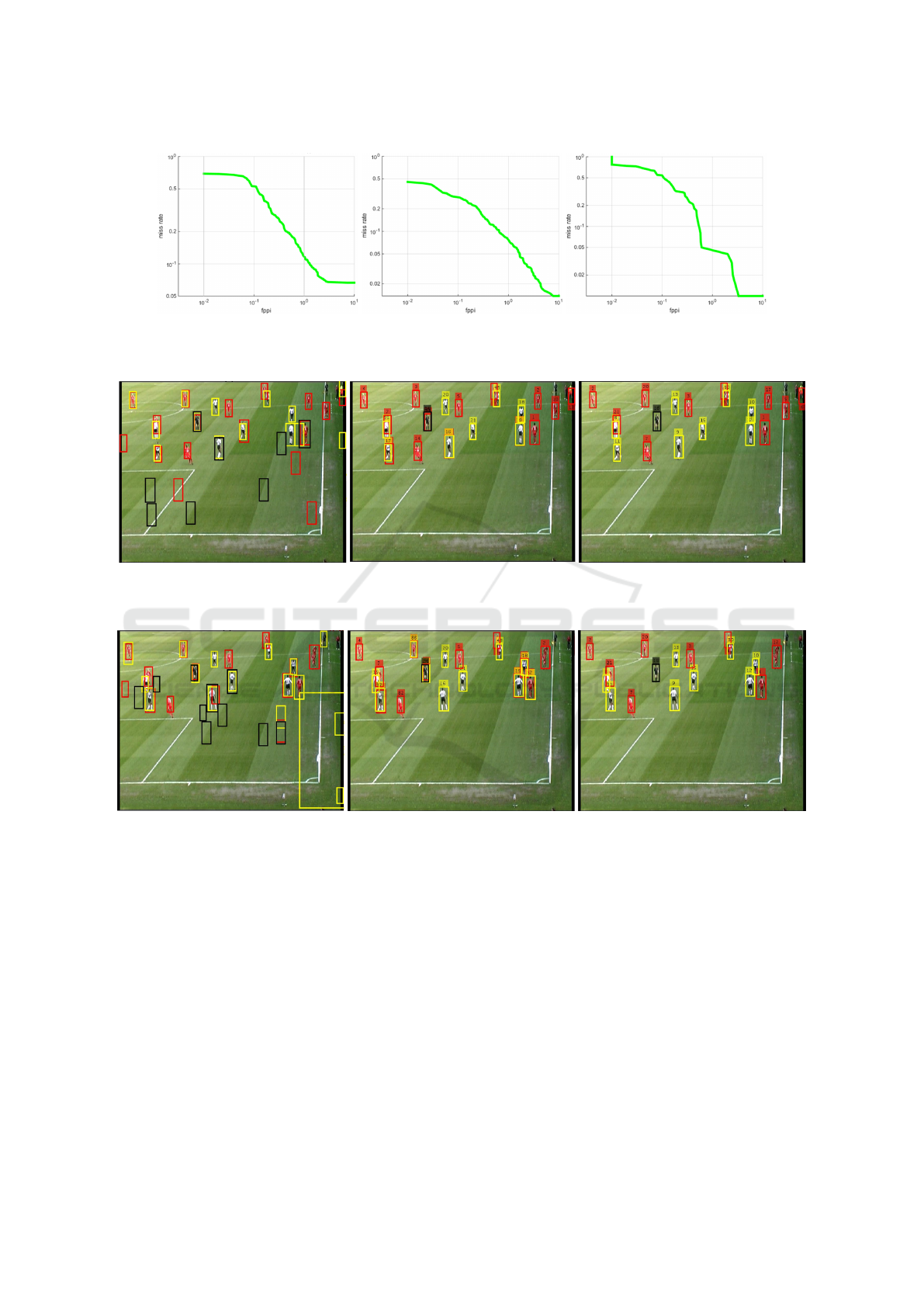
Figure 1: Extracting detection probabilities for three target types (red, white and referee) from ROCs of 3 detectors: red

team detector (left), white team detector (middle) and referee detector (right) when tested on red team instances, white team

instances and referee instances, respectively.

Figure 2: Results of detections (left), three independent GM-PHD trackers (middle) and tri-GM-PHD tracker (right), for frame

25.

Figure 3: Results of detections (left), three independent GM-PHD trackers (middle) and tri-GM-PHD tracker (right), for frame

57.

zero initial velocity are used as a mean of the Gaus-

sian distribution using a predetermined initial covari-

ance for birthing of targets, i.e. new targets are born

in the region of the state space for which the likeli-

hood will have high values. Very small initial weight

(e.g. 10

−4

) is assigned to the Gaussian components

for new births as this is effective for high clutter rates.

1,γ,k

= P

2,γ,k

= P

3,γ,k

= diag([100,100, 25,25,20, 20]).

(25)

We evaluate the tracking methodology of the tri-

GM-PHD tracker in comparison with ﬁrst, repeated

independent detection on each frame, and second,

with three independent GM-PHD trackers. Using the

football video sequence, the examples shown in Fig-

ures 2, 3 and 4 are for repeated detection (left), three

independent GM-PHD trackers (middle), and the tri-

GM-PHD tracker (right) for frames 25, 57 and 73, re-

spectively. Hence, Figure 3 (left) designates detec-

tions in which the red, white footballers and the ref-

eree are detected both correctly and incorrectly, i.e.

one object may be detected by many detectors. For

example, the referee is detected 3 times: by the red

team detector (red), by the white team detector (yel-

low) and the referee detector (black). Moreover, there

are many background false positives that arise from

our choice to set the detection probability high at the

expense of higher clutter. Using the three independent

VISAPP 2017 - International Conference on Computer Vision Theory and Applications

474

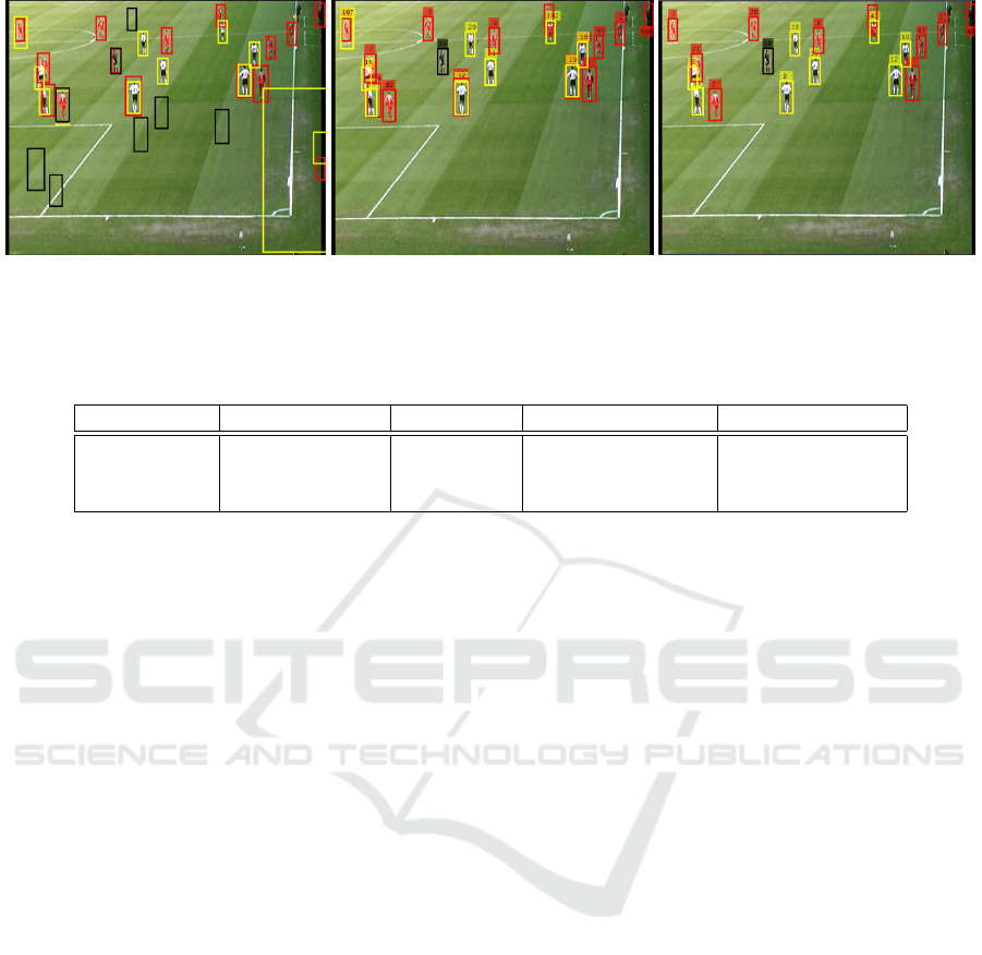
Figure 4: Results of detections (left), three independent GM-PHD trackers (middle) and tri-GM-PHD tracker (right), for frame

73.

Table 1: Frame-averaged cardinality and OSPA errors, time taken and discrimination rate at the extracted detection probabil-

ities for tri-GM-PHD ﬁlter, three independent GM-PHD ﬁlters and Detections.

Method Cardinality error OSPA error time taken discrimination rate

Detections 10.22 37.61 pixels 0.59 seconds/frame 0%

3 GM-PHDs 5.76 30.86 pixels 0.80 seconds/frame 0%

Tri-GM-PHD 0.11 10.59 pixels 3.00 seconds/frame 99.20%

GM-PHD trackers to effectively eliminate false pos-

itives, confused detections are not resolved as shown

in Figure 3 (middle). However, our proposed tri-GM-

PHD tracker effectively eliminates the false positives

and confused detections as shown in Figure 3 (right).

The tri-GM-PHD ﬁlter is evaluated quantitatively

for the whole test sequence and compared with three

independent GM-PHD ﬁlters and repeated detection

using cardinality, OSPA metric (Schumacher et al.,

2008), discrimination rate and time taken. We use

OSPA metric which is designed for evaluating RFS-

based ﬁlters rather than multi-object tracking accu-

racy (MOTA) (Bernardin and Stiefelhagen, 2008)

which is widely used for evaluating other traditional

multi-target tracking algorithms (Yoon et al., 2016;

Choi, 2015). Furthermore, our algorithm is devel-

oped not only for tracking but also for discriminat-

ing different target types overcoming their confusions

unlike algorithms such as (Yoon et al., 2016; Choi,

2015). Therefore, OSPA is the right evaluation met-

ric to evaluate our approach. The computational costs

arise from experiments on a i5 2.50 GHz core pro-

cessor with 6 GB RAM using Matlab and we ac-

knowledge that these are not deﬁnitive and give a

rough guide only. Though labeling of the targets us-

ing Munkres’s variant of the Hungarian assignment

algorithm works well as shown in Figures 2 (right), 3

(right) and 4 (right), we didn’t include this in our eval-

uation as it is not part of the quantitative comparison

of the ﬁltering and type labeling of either the detection

or distinct GM-PHD ﬁlters. We present the cardinal-

ity and OSPA error plots in Figure 5 (left) and Fig-

ure 5 (right) respectively, in red for ground truth (car-

dinality), green for the tri-GM-PHD ﬁlter, blue for the

three independent GM-PHD ﬁlters and magenta for

repeated detection. As summarised in Table 1 the av-

erage absolute cardinality error using detection only is

10.22, reduced to 5.76 using the standard GM-PHD

ﬁlter and to 0.11 using the tri-GM-PHD ﬁlter. The

overall frame-averaged value of OSPA error for the

tri-GM-PHD ﬁlter is 10.59 pixels, compared to three

independent GM-PHD ﬁlters of 30.86 pixels, and re-

peated detections of 37.61 pixels. The proposed ap-

proach reduces the cardinality and OSPA errors by a

large margin over three independent GM-PHD ﬁlters

and repeated detection, although this has more com-

putational cost as also shown in Table 1. Overall,

this demonstrates that our approach can effectively

discriminate true positives from clutter, while elimi-

nating confused detections with a discrimination rate

of 99.20%. The mis-discrimination rate of 0.80% oc-

curs primarily during the initial frames (e.g. the ﬁrst 7

frames) until the prediction-update process stabilises

and the true detections are conﬁrmed by the motion

between adjacent frames.

Figure 6 shows another example in which the in-

dividual footballers are detected, ﬁltered, tracked and

labeled for 100 frames. The image has been cropped

and and immediately follows a throw-in as the players

move away left from the touchline. The ﬁgures show

the individual tracks, the labels of the footballers and

the referee as small numbers over the targets. From

this sequence, we see for example that the red player

number 6 and the white player number 10, and several

others, are consistently tracked through the sequence.

However the labeling does occasionally make mis-

Multiple Target, Multiple Type Visual Tracking using a Tri-GM-PHD Filter

475

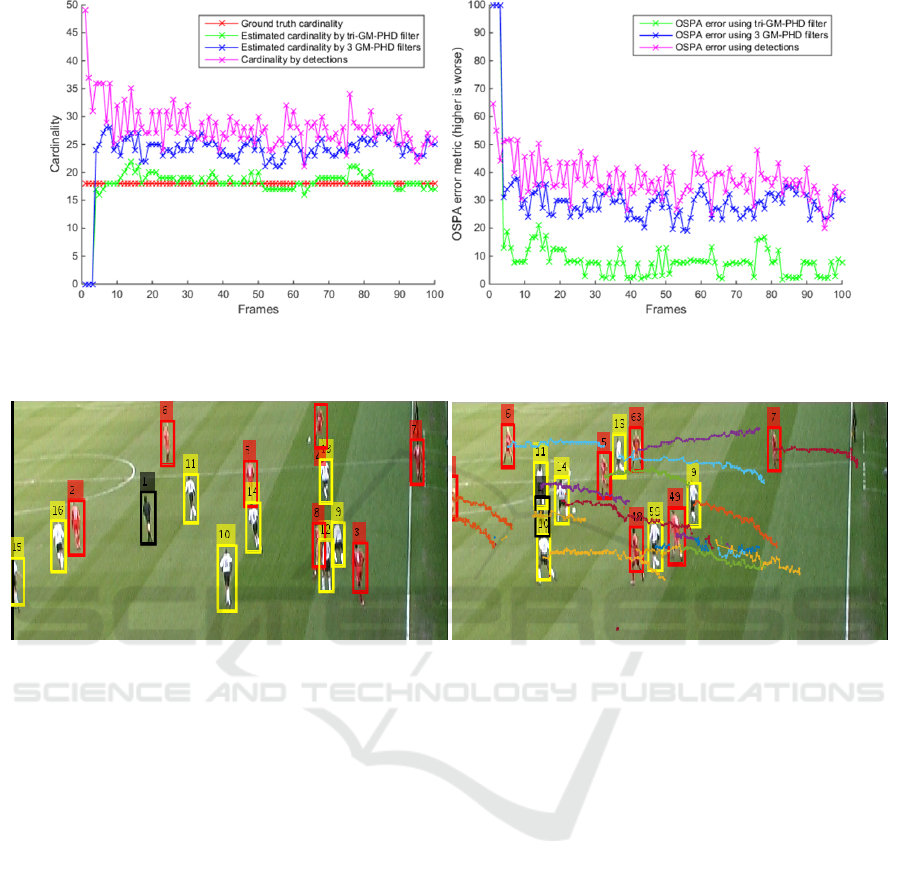
Figure 5: Cardinality error (left) and OSPA error (right): Ground truth (red for cardinality only), tri-GM-PHD ﬁlter (green),

three independent GM-PHD ﬁlters (blue), detections (magenta).

Figure 6: Tracking the red and white teams, and referee from frame 193 (left) to frame 293 (right).

takes, for example red player 3 who starts near the

touchline is ﬁnally labeled as red player number 49 in

frame 293. This is due to occlusion and lack of persis-

tence in the detection and tracking as it uses succes-

sive frames only, so that if a player disappears then

re-appears after several frames he is treated as a new

target. Nevertheless, although this evaluation is not

part of the Tri-GM-PHD ﬁlter, the labeling that we

apply has good performance with a mean label switch

error of only 0.43%.

6 CONCLUSIONS

We have developed an extension of the PHD ﬁlter

in the RFS framework to account for three different

types of multiple targets with separate observations

in the same scene, allowing for different probabilities

of detection, scene clutter and confusion between tar-

gets of different types at the detection stage. This ex-

tends the standard GM-PHD ﬁlter (Vo and Ma, 2006)

to a tri-GM-PHD ﬁlter. This has been evaluated us-

ing video sequences with the separate targets deﬁned

as different team players and the referee. We also ap-

plied Munkres’s variant of the Hungarian assignment

algorithm as data association on the ﬁltered results of

the ﬁlter as a post-process.

The key ﬁnding is that by considering and mod-

eling confusions between the different types of target

and detector we can improve the target discrimina-

tion rate, demonstrated by quantitative measurement

of cardinality and the OSPA score. In comparison

with separate PHD ﬁlters, as is usual practice, we can

reduce the mean absolute error in cardinality to less

than 1 target, with a corresponding reduction in the

OSPA location metric to a mean of 10.59 from 30.86

pixels. Application of the Hungarian labeling method

shows good data association so that we are able to

track individual targets over the sequence with a mean

label switch error of only 0.43. The work we have

done has shown that the tri-GM-PHD ﬁlter has poten-

tial both to track targets in video data, and to better

address multiple target confusions than the standard

method.

VISAPP 2017 - International Conference on Computer Vision Theory and Applications

476

ACKNOWLEDGEMENT

We would like to acknowledge the support of the

Engineering and Physical Sciences Research Council

(EPSRC), grant references EP/K009931, EP/J015180

and a James Watt Scholarship.

REFERENCES

Ahmed, E., Jones, M., and Marks, T. K. (2015). An

improved deep learning architecture for person re-

identiﬁcation. In The IEEE Conference on Computer

Vision and Pattern Recognition (CVPR), pages 3908–

3916.

Appel, R., Fuchs, T., Dollar, P., and Perona, P. (2013).

Quickly boosting decision trees – pruning under-

achieving features early. In ICML, volume 28, pages

594–602.

Bernardin, K. and Stiefelhagen, R. (2008). Evaluating mul-

tiple object tracking performance: The CLEAR MOT

metrics. J. Image Video Process., pages 1:1–1:10.

Bourgeois, F. and Lassalle, J.-C. (1971). An extension of

the munkres algorithm for the assignment problem to

rectangular matrices. Commun. ACM, 14(12):802–

804.

Cai, Y., de Freitas, N., and JJ, L. (2006). Robust visual

tracking for multiple targets. In IN ECCV, pages 107–

118.

Cham, T.-J. and Rehg, J. M. (1999). A multiple hypothesis

approach to ﬁgure tracking. In CVPR, pages 2239–

2245. IEEE Computer Society.

Choi, W. (2015). Near-online multi-target tracking with ag-

gregated local ﬂow descriptor. In The IEEE Interna-

tional Conference on Computer Vision (ICCV).

Dollar, P., Appel, R., Perona, P., and Belongie, S. (2014).

Fast feature pyramids for object detection. IEEE

Transactions on Pattern Analysis and Machine Intel-

ligence, 99:14.

Liu, J. and Carr, P. (2014). Detecting and tracking sports

players with random forests and context-conditioned

motion models. In Computer Vision in Sports, pages

113–132. Springer.

Maggio, E., Taj, M., and Cavallaro, A. (2008). Efﬁcient

multi-target visual tracking using random ﬁnite sets.

IEEE Transactions On Circuits And Systems For Video

Technology, pages 1016–1027.

Mahler, R. P. (2003). Multitarget bayes ﬁltering via ﬁrst-

order multitarget moments. IEEE Trans. on Aerospace

and Electronic Systems, 39(4):1152–1178.

Matzka, P., Wallace, A., and Petillot, Y. (2012). Efﬁcient re-

source allocation for automotive attentive vision sys-

tems. IEEE Trans. on Intelligent Transportation Sys-

tems, 13(2):859–872.

Pasha, S., Vo, B.-N., Tuan, H. D., and Ma, W.-K. (2009).

A gaussian mixture PHD ﬁlter for jump markov sys-

tem models. Aerospace and Electronic Systems, IEEE

Transactions on, 45(3):919–936.

Rasmussen, C. and Hager, G. D. (2001). Probabilistic data

association methods for tracking complex visual ob-

jects. IEEE Transactions on Pattern Analysis and Ma-

chine Intelligence, 23:560–576.

Ristic, B., Clark, D., and Vo, B.-N. (2010). Improved SMC

implementation of the PHD ﬁlter. In Information Fu-

sion (FUSION), 2010 13th Conference on, pages 1–8.

Ristic, B., Clark, D. E., Vo, B.-N., and Vo, B.-T. (2012).

Adaptive target birth intensity for PHD and CPHD ﬁl-

ters. IEEE Transactions on Aerospace and Electronic

Systems, 48(2):1656–1668.

Schumacher, D., Vo, B.-T., and Vo, B.-N. (2008). A con-

sistent metric for performance evaluation of multi-

object ﬁlters. Signal Processing, IEEE Transactions

on, 56(8):3447–3457.

Vo, B.-N. and Ma, W.-K. (2006). The Gaussian mixture

probability hypothesis density ﬁlter. Signal Process-

ing, IEEE Transactions on, 54(11):4091–4104.

Vo, B.-N., Singh, S., and Doucet, A. (2005). Sequential

monte carlo methods for multitarget ﬁltering with ran-

dom ﬁnite sets. IEEE Transactions on Aerospace and

Electronic Systems, 41(4):1224–1245.

Wei, Y., Yaowen, F., Jianqian, L., and Xiang, L.

(2012). Joint detection, tracking, and classiﬁcation

of multiple targets in clutter using the PHD ﬁlter.

Aerospace and Electronic Systems, IEEE Transac-

tions on, 48(4):3594–3609.

Yang, W., Fu, Y., and Li, X. (2014). Joint target tracking and

classiﬁcation via RFS-based multiple model ﬁltering.

Information Fusion, 18:101–106.

Yoon, J. H., Lee, C.-R., Yang, M.-H., and Yoon, K.-J.

(2016). Online multi-object tracking via structural

constraint event aggregation. In CVPR.

Zhou, X., Li, Y., He, B., and Bai, T. (2014). GM-PHD-

based multi-target visual tracking using entropy distri-

bution and game theory. Industrial Informatics, IEEE

Transactions on, 10(2):1064–1076.

Multiple Target, Multiple Type Visual Tracking using a Tri-GM-PHD Filter

477