A Robust Chessboard Detector for Geometric Camera Calibration

Mathis Hoffmann, Andreas Ernst, Tobias Bergen, Sebastian Hettenkofer and Jens-Uwe Garbas

Fraunhofer Institute for Integrated Circuits IIS, Am Wolfsmantel 33, 91058 Erlangen, Germany

Keywords:

Chessboard Detection, Camera Calibration, Endoscope Calibration, Integral Image, Checkerboard Detection.

Abstract:

We introduce an algorithm that detects chessboard patterns in images precisely and robustly for application

in camera calibration. Because of the low requirements on the calibration images, our solution is particularly

suited for endoscopic camera calibration. It successfully copes with strong lens distortions, partially occluded

patterns, image blur, and image noise. Our detector initially uses a sparse sampling method to ﬁnd some con-

nected squares of the chessboard pattern in the image. A pattern-growing strategy iteratively locates adjacent

chessboard corners with a region-based corner detector. The corner detector examines entire image regions

with the help of the integral image to handle poor image quality. We show that it outperforms recent solutions

in terms of detection rates and performs at least equally well in terms of accuracy.

1 MOTIVATION

Endoscopic procedures are frequently used in the

treatment of various diseases and internal injuries.

Minimally invasive surgery with endoscopic instru-

ments is performed, for example, on abdominal or-

gans (laparoscopy), joints (arthroscopy), or the brain

(neurosurgery). Endoscopy requires good orienta-

tion, coordination, and ﬁne motor skills of the sur-

geon. Therefore, computer systems that offer navi-

gation support to the physician are of increasing sig-

niﬁcance. Navigation systems that relate the view

through the endoscope to the geometry of the surgi-

cal site require a calibrated camera. In this context,

calibration refers to the process of estimating the in-

trinsic camera parameters. The intrinsic parameters

of a distorted pinhole camera model consist of the fo-

cal length, the principal point, as well as radial and

tangential distortions. Usually, camera calibration is

a two-step process: First, a known calibration pattern

is detected in the images. Second, the calibration pa-

rameters are estimated based on correspondences be-

tween points on the pattern and their projections in

the images. In this paper, we focus on the ﬁrst step.

We present a new method for detecting the calibration

target robustly and precisely under hard constraints.

Camera calibration for endoscopic applications

poses several challenges. Endoscopes often have

wide-angle lenses with typical viewing angles be-

tween 90° and 120°. Therefore, distortion effects are

very strong. Due to the optical setup of the endo-

scope, the light source is close to the optical cen-

ter. This often causes strong inhomogeneity, glare,

vignetting effects, and high image noise in badly il-

luminated regions. Within a clinical environment,

non-technical staff must be able to perform the cal-

ibration process quickly. Consequently, the calibra-

tion method must reliably handle motion blur, defo-

cussing, and recordings of partially captured patterns.

Various patterns have been developed. Still, the

planar chessboard pattern is most established. Mal-

lon et al. (Mallon and Whelan, 2007) have shown

that the chessboard pattern outperforms circle pat-

terns in the case of strong perspective or radial dis-

tortion. Self-identifying targets (like ARTags (Fiala

and Shu, 2005)) are more complex and require high

resolution and low-noise images. We will therefore

focus on a classical chessboard pattern. Nonetheless,

the proposed method can be adapted to other calibra-

tion targets as well.

2 RELATED WORK

A variety of calibration approaches have been pro-

posed to determine intrinsic camera parameters from

a set of images of a known calibration pattern. Sub-

stantial contributions include early works by Tsai

(Tsai, 1987), Heikkilä and Silven (Heikkila and Sil-

ven, 1997), and Zhang (Zhang, 2000). Various im-

provements and extensions of these methods have

been suggested for application in endoscopic camera

Hoffmann M., Ernst A., Bergen T., Hettenkofer S. and Garbas J.

A Robust Chessboard Detector for Geometric Camera Calibration.

DOI: 10.5220/0006104300340043

In Proceedings of the 12th International Joint Conference on Computer Vision, Imaging and Computer Graphics Theory and Applications (VISIGRAPP 2017), pages 34-43

ISBN: 978-989-758-225-7

calibration (Zhang et al., 2000; Wengert et al., 2006).

Moreover, alternative camera models have been sug-

gested, tailored to the optical setup of endoscopic

cameras (Stehle et al., 2007; Li et al., 2008). Bar-

reto et al. addressed the requirement of an easy-to-use

calibration process and developed a single-shot cal-

ibration method to allow for an endoscope calibra-

tion procedure with minimal effort for the surgeon

(Barreto et al., 2009). Ruﬂi et al. also proposed a

method for the detection of a calibration pattern (Ru-

ﬂi et al., 2008). Their approach is based on an adap-

tive thresholding of the input images, followed by a

binary contour ﬁnder to detect the quadrangles of a

chessboard pattern. A variation of this approach is im-

plemented in the OpenCV computer vision toolbox.

More recently, Placht et al. presented a chessboard de-

tection method (ROCHADE) for highly distorted im-

ages. They detect edges based on a gradient image

to create a graph representation of the detected chess-

board quadrangles. Graph-matching is then applied

to conﬁrm correct detection results. Both methods re-

quire the entire calibration pattern to be visible in the

image. This is a major drawback in the context of en-

doscopy. It impedes to capture chessboard corners in

the outer image regions, where barrel distortion has

the strongest effect. So, the most valuable image re-

gions cannot contribute any point correspondences.

Fuersattel et al. improved the ROCHADE method to

also handle partially visible chessboards by including

a subgraph-matching strategy (called OCPAD). Sun

et al. proposed a chessboard detection algorithm that

locates corners robustly under inhomogeneous illumi-

nation and also handles deformed chessboards (Sun

et al., 2008). They detect corner points by evaluating

bright and dark sequences along circles around corner

point candidates.

Most of the established approaches either apply

a binarization procedure to separate dark and bright

regions or extract edges from the images to localize

chessboard corners. In contrast, we propose to eval-

uate region statistics to robustly and accurately detect

chessboard corners under difﬁcult image conditions.

Considering entire image regions (corresponding to

chessboards quadrangles) makes the approach insen-

sitive to image noise and blurry edges. Our method is

explicitly designed to handle partially visible chess-

boards with strong distortion effects under inhomo-

geneous illumination.

3 PROPOSED METHOD

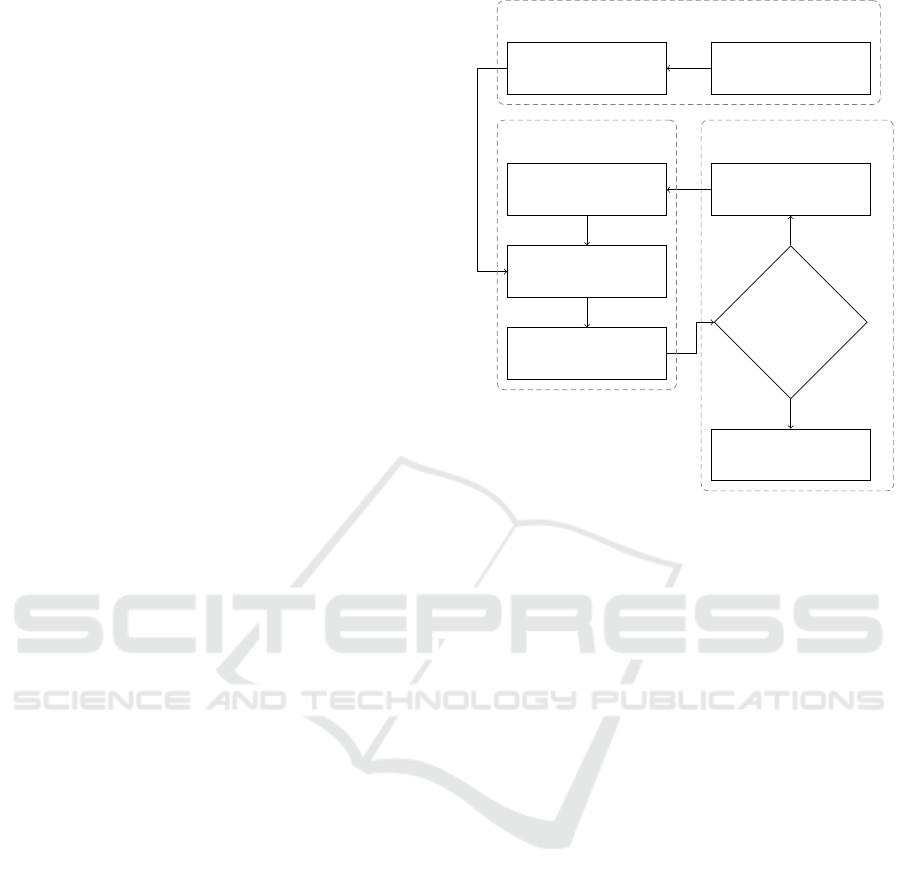
Figure 1 shows an overview of our method. The in-

dividual steps are illustrated in Figure 2. The process

sparse region

sampling

select best

create candidates

locate corners

select candidates

reestimate model

parameters

found new

corners?

done

yes

initial estimation

pattern growing parameter optimization

Figure 1: Overview of the proposed method. The process

is divided into an initial estimation, a pattern growing and a

parameter optimization phase.

consists of three phases. The initialization phase uses

a sparse sampling strategy to ﬁnd an initial guess for

the chessboard position and size (Figures 2a and 2b).

The guess is then improved to subpixel precise corner

locations and allows an initial camera parameter esti-

mation (Figure 2c). The pattern-growing phase itera-

tively searches new chessboard corners in the vicinity

of detected corners and updates the camera parame-

ters in the optimization phase (Figures 2d to 2f). The

following sections explain the three phases in detail.

3.1 Initial Estimation

Our method requires an initial estimate of the chess-

board size, pose and position. Therefore, we regularly

scan the image with a 3 × 3 chessboard model to ﬁnd

positions of high correspondence between the model

and the image (Figures 2a and 2b).

At each position, we sample the intensities of 5

points within each of the 9 chessboard patches (see

Figure 3). The regular structure of a chessboard al-

lows us to divide it into two groups of homogeneous

intensities. A successful initial guess is characterized

by a high intensity difference between both groups

and a low intensity variance within each group. The

Fisher linear discriminant is suited to identify the best

guess. It is commonly used to maximize the spread

of samples in pattern classiﬁcation problems (Duda

et al., 2001). Let

and

denote the standard de-

A Robust Chessboard Detector for Geometric Camera Calibration

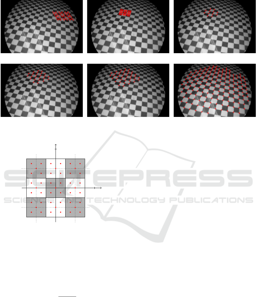
(a) Arbitrary sample (b) Accepted sample (c) Initially located corners

(d) One iteration (e) Two iterations (f) Convergence after 14 iterations

Figure 2: Individual steps of our method.

(2, 0)

(0, 2)

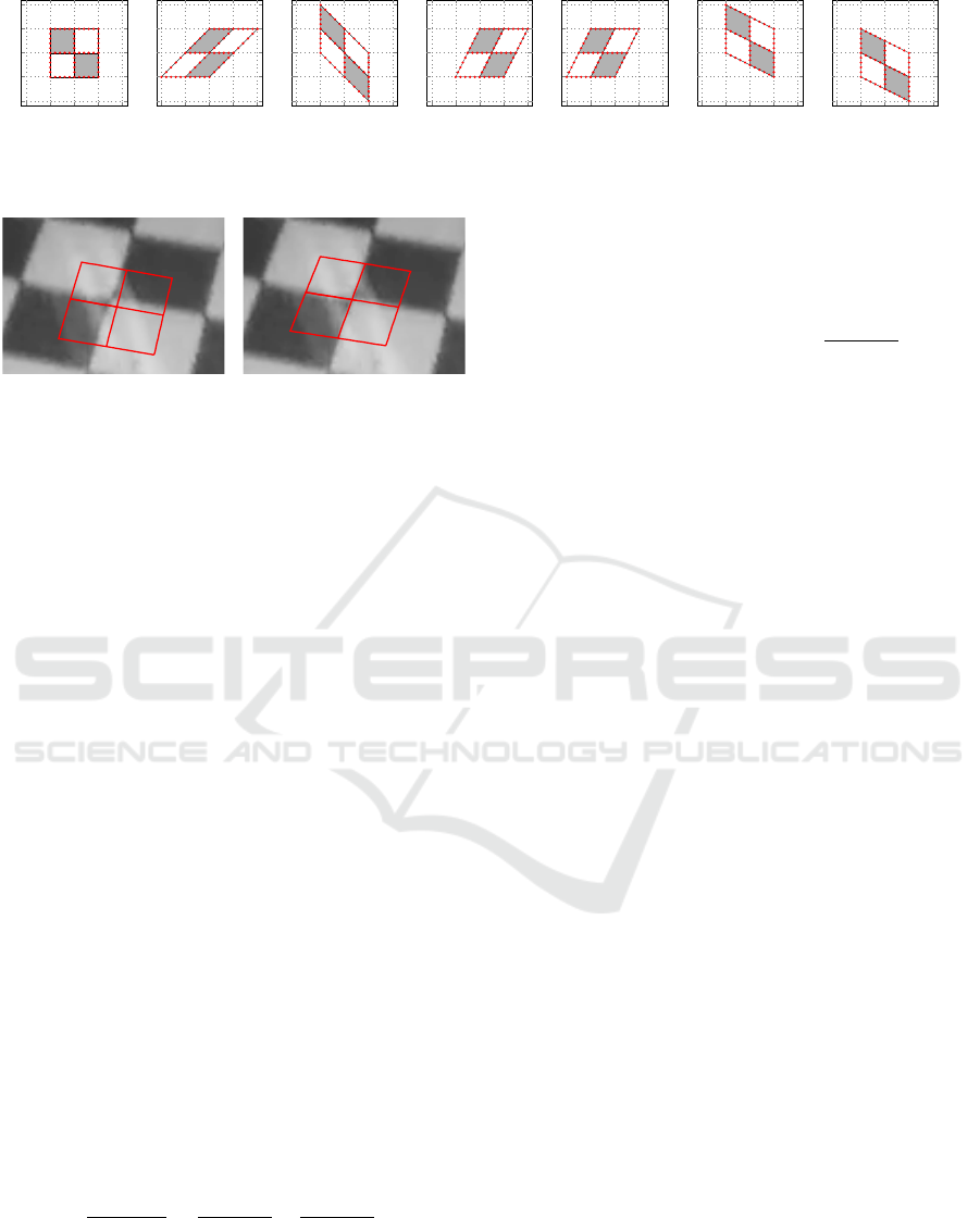
Figure 3: Sparse sampling model. Red points indicate sam-

pling coordinates. The grid size is 1 in x and y direction.

Note that the model consists of two groups of homogeneous

regions (black and white).

viation of all samples in the respective group. Let ˆµ

and ˆµ

denote the corresponding intensity means. We

deﬁne the correspondence between the chessboard

model and the image based on the idea of the Fisher

discriminant as

ˆµ

− ˆµ

, (1)

where p denotes the dependency on the model pa-

rameters, i.e. size, pose, and position. We test for

different combinations of size, position, shearing and

rotation to ﬁnd a proper guess. Finally, we choose

the sample that maximizes |s

| and calculate an initial

homography H

based on correspondences between

the model and image coordinates. We do not yet ac-

count for distortion and initialize the distortion d

an identity mapping. We denote the complete proce-

dure as sparse region sampling.

3.2 Pattern Growing

The initial estimate provides an approximation of H

and d

that is valid in a close vicinity to the initial

guess. We use the approximation to predict corner

locations of the sparse sampling model in the image.

We drop the four outer corners of the sparse sampling

model (see Figure 3), because their prediction is often

less accurate and locate the remaining 12 corners with

subpixel accuracy using the corner detector depicted

in the following sections. Figure 2c shows the result

of this step. The update of the projection parameters

yields H

and d

. Then, we iteratively search nearby

chessboard corners until we can’t detect any new cor-

ner. Therefore, we consider the four direct neighbors

of the chessboard corners that have already been de-

tected and apply the corner detector to each of them.

We append the new corners to the set of detected cor-

ners on success and drop them otherwise. After every

iteration, we update H and d to improve the projection

parameters for the next iteration.

Let us give an example: In the ﬁrst iteration, we

consider the neighbors of the 12 initial corners. As-

sume, we begin with v

= (0.5, 1.5)

of Figure 3. The

four direct neighbors of v

are given by

n(v

)



± 1





± 1



. (2)

We apply the corner detection only to the new points

(1.5, 1.5)

and (0.5, 2.5)

and add them to the set of

VISAPP 2017 - International Conference on Computer Vision Theory and Applications

detected corners on success. We apply this procedure

to all 12 points and subsequently update the projec-

tion parameters to get H

and d

. The result of this

iteration is shown in Figure 2d.

The pattern-growing phase relies on the region-

based corner detector introduced in Section 3.2.3. It

makes our method robust against noise and blur. First,

we introduce a morphable model in Section 3.2.1 and

its projection into the image space in Section 3.2.2 to

explain the corner detector in detail.

3.2.1 Morphable Corner Model

The morphable model is deﬁned by a linear combi-

nation of N deformed templates T

with coefﬁcients

and an undeformed template T

. The coefﬁcients

determine the shape of the model. Each template con-

sists of M vertices

and is deﬁned by













, with k ∈ [0,N]. (3)

We associate one parameter α

with each deformation

target T

for k > 0 to specify the weight of each tem-

plate in the linear combination. In addition, we intro-

duce global translation and scaling parameters ∆

, ∆

and s. The morph parameter vector combines all pa-

rameters in

= (∆

, ∆

, s, α

, . . . , α

) (4)

and parametrizes the morphable model m:

m: R

N+3

→ R

M×2

p 7→ M =







˘x

˘y

˘x

˘y







= s

∑

k=1

− T

)







∆







(5)

In this work, we use the elementary templates

shown in Figure 4. Some of the illustrated shearing

templates do not introduce additional deformations.

However, they enable identical deformations by di-

verse parameter combinations and simplify alignment

to the chessboard corners. Experiments conﬁrmed a

better convergence with these additional templates.

The morphable model is inﬂuenced by the point

distribution model (pdm) proposed by Cootes and

We denote unmorphed coordinates in model space by

(x, y) and morphed coordinates in model space by ( ˘x, ˘y).

Further, we denote image coordinates by (u, v), their ho-

mogeneous representations by ( ˜u, ˜v, ˜w) and distorted image

coordinates by ( ˘u, ˘v).

Taylor (Cootes and Taylor, 1992). The deviation of

each deformation template from the default template

is similar to the statistical modes of variation in the

pdm. However, we deﬁne the deformation templates

manually and add scaling and translation in the model

coordinate frame.

3.2.2 Projection Model

The morphable model resides in the model coordinate

frame and M is a matrix of model coordinates. We

use planar calibration targets. Therefore, the image

coordinates of the model lie in a two dimensional lin-

ear manifold of R

. A homography deﬁnes the linear

projection of each vertex ( ˘x, ˘y) from M into the image

frame by





˜u

˜v

˜w





= H





˘x

˘y





. (6)

The homography matrix H ∈ R

3×3

is deﬁned up to

scale (Zhang, 2000). We get the inhomogeneous

representation of the image coordinates by u = ˜u/ ˜w

and v = ˜v/ ˜w, respectively. Afterwards, we apply the

Brown-Conrady model to account for non-linear ra-

dial and tangential distortion (Brown, 1971):

˘u

= u



1 + k

+ k





+ 2u



+ 2p



˘v

= v



1 + k

+ k





+ 2v



+ 2p



where the coefﬁcients k

, k

cause radial distortion

and p

, p

cause tangential distortion. The radius r

is the distance of each vertex to the distortion center

, c

= (u − c

)

+ (v − c

)

The distortion parameter vector summarizes all coef-

ﬁcients in d

= (c

, c

, k

, p

). We combine

the linear and non-linear transform in

: R

N+3

× R

3×3

× R

→ R

M×2

(p, H, d) 7→ M







˘u

˘v

˘u

˘v







. (7)

The number of coefﬁcients used for distortion

modeling inﬂuences the accuracy of the model. Tsai

shows that a radial distortion model with one coefﬁ-

cient is sufﬁcient for industrial machine vision appli-

cations (Tsai, 1987). Barreto et al. show that more

than a single radial distortion coefﬁcient can be ad-

vantageous for endoscopy applications (Barreto et al.,

2009). We focus on endoscopy images with strong

distortion effects. Therefore, we use two radial and

two tangential coefﬁcients, similar to others (Zhang,

2000; Wei and Ma, 1994).

A Robust Chessboard Detector for Geometric Camera Calibration

Figure 4: Different morph templates. T

: unmorphed template; T

and T

: shearing at the model center; T

- T

: shearing

by moving only the top, bottom, left and right side.

Figure 5: Subpixel precise corner detection using a 2 × 2

corner model. The corner model is shown before (left) and

after (right) optimization.

3.2.3 Region-based Corner Detection

Our morphable corner detection model M

consists

of four distinct regions that form a 2 × 2 chessboard

pattern (see Figure 5). The outline of each region is

given by a sequence of vertices ( ˘u

, ˘v

), i ∈ [k

] with

> k

+ 2 and k

r+1

= l

+ 1 for all r ∈ [1,4]. Here,

r denotes the region index and k

, l

∈ [1,M] are the

boundaries of region r. We apply the 2 × 2 corner

model to the domain of corner detection. Therefore,

we need a criterion that measures how well the model

separates the four chessboard regions in the image. In

Section 3.1, we applied a variant of the Fisher dis-

criminant to ﬁnd the sample that separates the groups

of black and white chessboard patches best. Based on

the same idea, we derive a local measure that provides

better guidance to the optimizer for subpixel precise

corner detection. We use the Levenberg-Marquardt

method to minimize the model residual. Therefore,

we split the Fisher discriminant into two indepen-

dent terms, where each term accounts for the variance

within one region and the separation of that region

from one of its neighbors. In contrast to the original

formulation, we use signed values to provide better

guidance to the optimizer. Finally, we turn the maxi-

mization into a minimization problem.

Let µ

and σ

be the pixel value mean and the stan-

dard deviation of all pixels in region r. We deﬁne the

separation between two regions r

and r

+ σ

− µ

We assume that the four regions are indexed in clock-

wise order, such that

, r

) ∈

{

(1, 2), (2, 3), (3, 4), (4, 1),

(2, 1), (3, 2), (4, 3), (1, 4)

}

denote pairs of neighboring regions. Then, we get the

separation of some region r

to one of its neighbors r

ˆe : [1,4] × [1,4] → R

, r

) 7→ e

− µ

(8)

Finally, we deﬁne the separation objective for M

= (e

, e

)

. (9)

For now, let us assume that we roughly know the

parameters H and d for the projection of M into the

image space. Therefore, we can predict the approx-

imate locations of the model coordinates (∆

, ∆

) in

the image. In the ﬁrst iteration, H and d are initialized

as described in Section 3.1. In subsequent iterations,

these estimates are updated by taking newly detected

corners into consideration. We describe the update

procedure in Section 3.3.

We search for the exact image location v

∗

( ˘u

∗

, ˘v

∗

) of the chessboard corner. This is done by min-

imizing e with respect to the morph template parame-

ters while keeping H and d constant. Therefore

∗

= arg min

kek

, (10)

where p is initialized with (∆

, ∆

, s, 0, . . .). We allow

the model to be translated and sheared with six differ-

ent shearing templates. This simpliﬁes minimization

because it lowers the risk that the error only decreases

when several parameters are adjusted simultaneously.

The solution, v

∗

is then given by the center vertex of

∗

,H,d) (see Figure 5).

Note that the scale parameter s of the model con-

trols the size of the 2 × 2 search template relative to

the chessboard size. We use s = 0.5, that is, each

patch of the search template covers approximately a

quarter of the area of the chessboard patch. If the cor-

ner detector fails with this conﬁguration (possibly be-

cause the point is located close to the image border),

we reduce s and try it again.

Applying the morph parameters in the model co-

ordinate frame makes them scale independent. For

example, adding 1 to ∆

always moves the template

by the width of one chessboard patch in the image

frame, independent of the image resolution and patch

size in the image. This allows ﬁxed delta values to

compute the numerical derivative of Equation (9).

VISAPP 2017 - International Conference on Computer Vision Theory and Applications

Figure 6: Examples of candidates that have been dropped

due to a degenerate result (left) or a high residual (right).

3.2.4 Candidate Selection

In some cases, the corner detector provides invalid lo-

cations in the image as shown in Figure 6. There-

fore, we introduce constraints that allow us to reject

invalid results. First, the detected corner must be in

the vicinity of the corner that is predicted by the cur-

rent model state. This ensures that the optimization

did not converge to a neighboring point. In practice,

it is sufﬁcient to allow a deviation of one half of the

chessboard patch width. This can be easily veriﬁed

with the translation parameters (∆

, ∆

) of m. They

must not differ more than 0.5 from their initialization.

Second, the area of the corner detection model be-

fore the optimization must not differ too much from

the area after optimization. This constraint prohibits

degenerate conﬁgurations. Finally, the residual error

kek

must meet the detection threshold. This rejects

chessboard corners on the border or outside of the pat-

tern.

3.2.5 Region Statistics

The calculation of µ

and σ

is done multiple times in

every iteration of the optimization. Therefore, it re-

quires a very fast algorithm. Ernst et al. have extended

the integral image approach of Viola and Jones (Vi-

ola and Jones, 2001) to approximate statistics within

polygonal image regions very efﬁciently (Ernst et al.,

2013). We summarize the method in the following.

The integral image I

of an image I is given by

(x,y)

∑

i6x, j6y

I(i, j). (11)

The sum of pixel values s

within some polygonal re-

gion r in an image of size w × h is approximated by

ˆs : R

M×2

× R

w×h

→ R



, I



7→ s

∑

i=k

( ˘u

, ˘v

i+1

)

−I

( ˘u

i+1

, ˘v

)],

(12)

with l

+ 1

= k

. Similary, ˆa provides the area a

in-

side r:

ˆa : R

M×2

→ R

7→ a

∑

i=k

( ˘u

˘v

i+1

− ˘u

i+1

˘v

(13)

Equations (12) and (13) allow the approximation of

the mean pixel value µ

within r by

ˆµ : R

M×2

× R

w×h

→ R



, I



7→ µ

(14)

Approximating the standard deviation σ

within r

requires a second integral image





, where each

pixel value is squared before the summation:

σ : R

M×2

× R

w×h

× R

w×h

→ R



, I







7→ σ

ˆs (M

, [I

]

)

− µ

. (15)

The efﬁcient approximation of µ

and σ

allows a

fast implementation of the robust local corner detec-

tor depicted in Section 3.2.3. Subpixel precision is

achieved by bilinear sampling. We refer to the pre-

vious work for a detailed explanation of the method

(Ernst et al., 2013).

3.3 Parameter Optimization

The corner detector ﬁnds the image location of a

chessboard corner v

∗

that corresponds to a corner co-

ordinate v

v = (∆

, ∆

) in model space. With that rela-

tion, we deﬁne two sets

{

, v

, . . . , v

}

and



∗

, v

∗

, . . . , v

∗



Here, v

denotes the model coordinate corresponding

to v

∗

and t ∈ N denotes the iteration number of the

pattern-growing step.

We apply Equation (7) with (H

, d

) on every

∈ M

to predict the image locations v

with the cur-

rent projection model. The parameter optimization

step aims at improving the projection model by mini-

mizing the errors between the detected corners v

∗

and

the predicted corners v

. Therefore, we ﬁnd the model

parameters for the next iteration by

t+1

, d

t+1

) = arg min

)









−v

∗

−v

∗









. (16)

A Robust Chessboard Detector for Geometric Camera Calibration

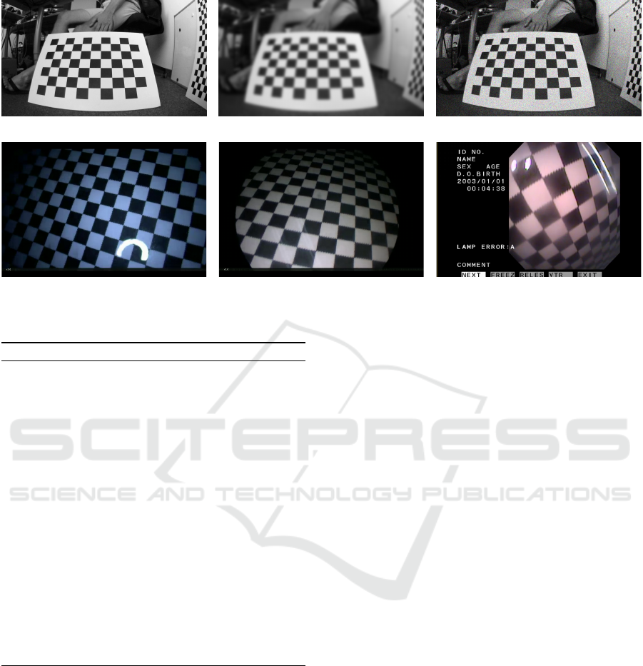
(a) Original OCPAD dataset (b) With b = 8 (c) With n = 16

(d) Wolf laparoscope (e) Wolf cystoscope (f) Olympus rhinolaryngoscope

Figure 7: Example images of the datasets.

Algorithm 1: Chessdetect.

1: M

← {v

, v

, . . . , v

}

2: t ← 0

3: Initialize H

and d

as described in Section 3.1

4: repeat

5: I

← {}

6: for all v

v ∈ M

7: Find p

∗

using (10)

8: v

∗

← center vertex of M

∗

9: if constraints are met then

10: I

← I

∪v

∗

11: else

12: M

← M

13: end if

14: end for

15: Find H

t+1

and d

t+1

using (16)

16: M

t+1

← M

∪ {n(v

v) |v

v ∈ M

}

17: t ← t + 1

18: until

t−1

t−2

3.4 Summary

We have introduced all relevant parts of our method

and summarize the procedure in Algorithm 1. To sim-

plify notation, we skip the algorithm for the initial

guess. Figure 3 shows our sparse sampling model and

Figure 2c shows an example of the initial corners.

Line 1 initializes M

with the corners of the sparse

sampling model. Line 3 initializes H

with the result

of the initial guess and sets d

to an identity map-

ping (see Section 3.1). The ﬁrst iteration locates the

corners M

of the sparse sampling model with sub-

pixel precision. The subsequent iterations search for

chessboard corners in the vicinity of already detected

corners (see Figures 2d to 2f). The algorithm iterates

until no new corners are detected.

Line 7 applies the region-based corner detector.

Subsequently, line 8 extracts the center vertex of the

corner model. Line 9 checks the constraints of Sec-

tion 3.2.4. On success, the point is accepted in line 10.

After all candidates in M have been detected or

dropped, the model parameters are estimated with the

updated correspondences in line 15. Finally, line 16

generates new candidates for the next iteration.

In practice, it is sufﬁcient to locate only the cor-

ners v

∈ M that are new in the current iteration. In

this case, it is recommended to locate all corners again

after the algorithm terminated, using the projection

parameters of the last iteration. Sometimes, the cor-

ner detector locates new corners in later iterations that

have been dropped before. This is caused by more

accurate projection parameters in later iterations that

lead to a better initialization of the corner model in

terms of translation and deformation.

4 EXPERIMENTS AND RESULTS

We evaluate our method with respect to image blur,

image noise, and only partially visible patterns. In

addition, we compare the performance with the Oc-

cluded Checkerboard Pattern Detector (OCPAD) by

Fuersattel et al. (Fuersattel et al., 2016). To the best

of our knowledge, this is the most recent approach

that can also cope with partially visible patterns.

VISAPP 2017 - International Conference on Computer Vision Theory and Applications

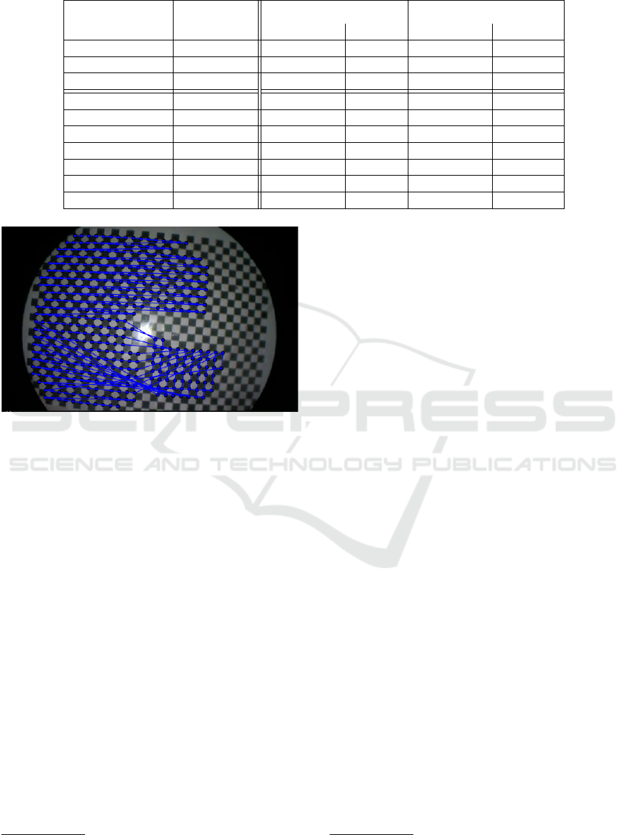
Table 1: Quantitative detection results.

set total images

detected images average points per image

Our method OCPAD Our method OCPAD

Endoscope set 1 99 90 71 204.3 99.9

Endoscope set 2 97 88 47 171.3 108.8

Endoscope set 3 100 79 38 128.0 64.7

OCPAD original 64 64 63 53.9 53.7

blur = 2 64 64 64 54.0 54.0

blur = 4 64 64 61 53.3 53.6

blur = 8 64 13 0 39.1 0.0

noise = 4 64 64 58 53.9 53.3

noise = 8 64 64 30 53.9 51.4

noise = 16 64 59 0 51.8 0.0

Figure 8: An image from endoscope set 1 that was discarded

manually, because OCPAD delivers false correspondences.

4.1 Datasets

Fuersattel et al. created datasets that consist of fully

visible as well as occluded chessboard patterns and

made them publicly available. In a ﬁrst step, we cre-

ated variants of their fully visible checkerboard pat-

terns dataset by artiﬁcially adding blur and noise to

show how our method performs under these circum-

stances in a reproducible environment. We applied

mogrify

on the dataset and used the following pa-

rameters:

• mogrify -blur 0xb

blurs an image. Here, b denotes the standard devi-

ation of the blur kernel. We use blur kernels with

a standard deviation of 2, 4 and 8.

• mogrify -attenuate n +noise gaussian

adds noise to an image. Here, n is the noise inten-

sity. We use noise intensities of 4, 8 and 16.

To reduce evaluation times, we only use the ﬁrst

64 images of the dataset. Otherwise, the OpenCV

calibrateCamera function used for the evaluation

http://www.imagemagick.org/script/mogrify.php

procedure in Section 4.2 takes very long. Examples

of the datasets are shown in Figures 7a to 7c.

The good image quality of the OCPAD datasets

and the low requirements on the chessboard detector

impede differentiation of both methods on the original

data. Although we raised the requirements by adding

noise and blur, we know that the results on the arti-

ﬁcially downgraded data do not necessarily general-

ize on real data. Therefore, we additionally compiled

datasets that put high requirements on the chessboard

detector using three different endoscopes:

• Set 1 was captured with a Panoview rigid laparo-

scope from Richard Wolf GmbH with 30

◦

side

view and a diameter of 10 millimeters.

• Set 2 was captured using a 0

◦

, 4 millimeter

Panoview rigid cystoscope from Richard Wolf

GmbH.

• Set 3 was captured with a 3.9 millimeter video rhi-

nolaryngoscope (Olympus ENF-VH). In contrast

to the previous endoscopes, it has a ﬂexible tube,

where the image sensor is located at the distal end

of the tube (chip-on-tip).

Figures 7d to 7f show example images of the datasets.

Each endoscopy dataset consists of 100 images.

4.2 Procedure

We processed every image in the datasets with both

chessboard detectors. Unfortunately, the OCPAD im-

plementation

requires to deﬁne the chessboard size

in advance. It uses this knowledge to reject images,

where only a small portion of the chessboard was de-

tected. We do not have this prior knowledge for the

endoscopy datasets, because the portion of the chess-

board that is visible varies a lot within the sequences.

Therefore, we choose the following strategy: First,

http://www.metrilus.de/blog/portfolio-items/ocpad/

A Robust Chessboard Detector for Geometric Camera Calibration

4 8

0.2

0.4

0.6

0.8

Endoscope set 1

2 4 8

0.2

0.4

0.6

0.8

Endoscope set 2

2 4 8

0.2

0.4

0.6

0.8

Endoscope set 3

2 4 8

0.1

0.15

0.2

0.25

0.3

0.35

0.4

0.45

OCPAD with blur

2 4 8

0.1

0.15

0.2

0.25

0.3

0.35

0.4

0.45

OCPAD with noise

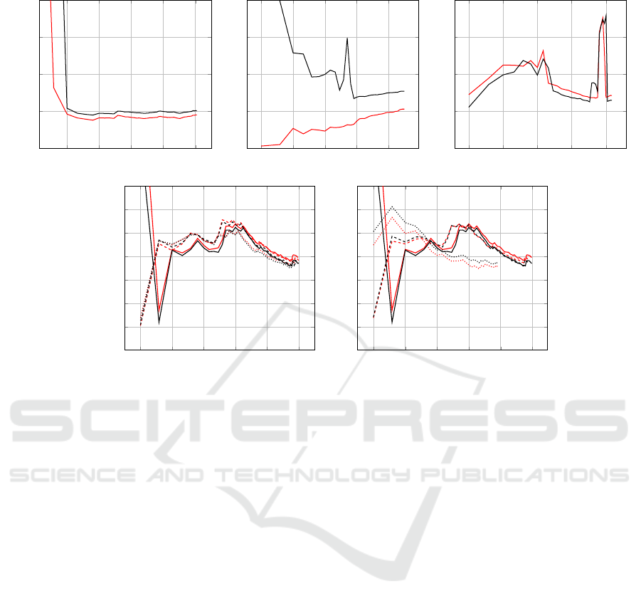
Figure 9: Average reprojection error µ of all images in the test sets. The camera parameters have been estimated with n

images. The plots show the results of our region-based detector (red) and the OCPAD detector (black). In case of the datasets

with artiﬁcial blur and noise, the solid lines correspond to the original data without blur or noise, whereas the dashed lines

correspond to the sets with b = 2 or n = 4 and the dotted lines correspond to b = 4 or n = 8. Unfortunately, we have no

results for b = 8 and n = 16, because OCPAD failed completely on these sets. Note, that the n-axis has a logarithmic scale

and that the scale of the µ-axis varies between the endoscope and the OCPAD sets.

we apply OCPAD and set the chessboard size to 4×4.

If it succeeds, we increase the chessboard size by 1 in

both dimensions and apply it again. We repeat this

until OCPAD fails and keep the last valid result.

In rare cases, OCPAD fails with an exception or

generates results that are obviously wrong (see Fig-

ure 8 for an example). In those cases, we simply re-

move the image from our datasets, such that it is com-

pletely ignored during the evaluation.

Based on the remaining results, we evaluate the

detection rates and the number of point correspon-

dences that have been found within each set. We only

consider images, where the corresponding method

has found at least 10 point correspondences. The de-

tection rate is deﬁned as the number of images (with

at least 10 detected point correspondences) in rela-

tion to the total number of images. We also evaluate

the average number of points that have been found in

each image. Finally, we evaluate the calibration ac-

curacy of both methods. To this end, we extract the

set of points that have been detected by both methods

and use them to estimate the camera parameters with

the OpenCV library. The function calibrateCamera

returns the ﬁnal average reprojection error. The repro-

jection error does not only depend on the calibration

and corner detection accuracy, but also on the quality

of the camera model. However, the error imposed by

the camera model exists in both methods.

4.3 Results

Table 1 summarizes the detection results of both

methods. On the endoscope datasets, our method pro-

vides signiﬁcantly higher detection rates and detects

roughly twice as much point correspondences per im-

age. On the artiﬁcially blurred images, both methods

perform approximately equally well until the standard

deviation reaches 8 pixels. In this case, the detection

rates of both methods drop. On the noisy images, the

detection rates of our method are approximately con-

stant, whereas the detection rates of OCPAD decrease

constantly.

Figure 9 shows the mean reprojection error for an

increasing number of images on all datasets. We dis-

cuss the peculiarities of the results in more detail. En-

doscope set 1 shows a high decrease of the reprojec-

tion error between 2 and 3 images with both methods.

An insufﬁcient number or inappropriate conﬁguration

VISAPP 2017 - International Conference on Computer Vision Theory and Applications

of correspondences in image 1 and 2 could explain

this effect with a poor calibration. Note, that we used

only the subset of correspondences that was detected

by both methods for a fair evaluation of the reprojec-

tion error. The sudden increase of the error in endo-

scope set 3 around image 28 is probably caused by the

image sequence, because the images that are added at

that point are taken from a very different perspective.

Overall, our method provides signiﬁcantly better

detection rates on difﬁcult endoscopy images as well

as in presence of artiﬁcial noise and performs equally

well in terms of accuracy on all datasets. Note, that

the accuracy of our corner detector depends on the

quality of the camera model. A more precise distor-

tion model can lead to a more realistic deformation of

the template in the image and a better alignment to the

corner.

5 CONCLUSIONS

We introduced a new method that detects chess-

board corners robustly and accurately even in pres-

ence of noise, blur and strong radial distortion. We

showed that the region-based corner detector com-

bined with the pattern-growing strategy detects signif-

icantly more chessboard corners then another recent

approach in difﬁcult images and performs equally

well in terms of accuracy. Our method is well suited

when the calibration pattern is only partially visible

or when the image quality is low. Therefore, it is

particularly qualiﬁed for endoscope calibration. The

method can be implemented efﬁciently using an ex-

tended variant of the integral image to calculate re-

gion means and variances. Due to its efﬁciency and

accuracy, it is well suited for clinical environments,

although it is not limited to that application.

REFERENCES

Barreto, J., Roquette, J., Sturm, P., and Fonseca, F. (2009).

Automatic camera calibration applied to medical en-

doscopy. In Proceedings of the British Machine Vision

Conference.

Brown, D. C. (1971). Close-range camera calibration. Pho-

togrammetric Engineering, 37.

Cootes, T. F. and Taylor, C. J. (1992). Active shape models -

’smart snakes’. In Proceedings of the British Machine

Vision Conference.

Duda, R. ., Hart, P. E., and Stork, D. G. (2001). Pattern

Classiﬁcation. Wiley, 2nd edition.

Ernst, A., Papst, A., Ruf, T., and Garbas, J.-U. (2013).

Check My Chart: A Robust Color Chart Tracker for

Colorimetric Camera Calibration. In Proceedings of

the 6th International Conference on Computer Vision

/ Computer Graphics Collaboration Techniques and

Applications.

Fiala, M. and Shu, C. (2005). Fully automatic camera

calibration using self-identifying calibration targets.

Technical report, National Research Council Canada.

Fuersattel, P., Dotenco, S., Placht, S., Balda, M., Maier, A.,

and Riess, C. (2016). OCPAD – Occluded Checker-

board Pattern Detector. In Proceedings of the IEEE

Winter Conference on Applications of Computer Vi-

sion.

Heikkila, J. and Silven, O. (1997). A four-step camera cal-

ibration procedure with implicit image correction. In

Proceedings of the Conference on Computer Vision

and Pattern Recognition.

Li, W., Nie, S., Soto-Thompson, M., Chen, C.-I., and A-

Rahim, Y. I. (2008). Robust distortion correction of

endoscope. In Proceedings of the International Soci-

ety for Optical Engineering.

Mallon, J. and Whelan, P. F. (2007). Which pattern? Bias-

ing aspects of planar calibration patterns and detection

methods. Pattern recognition letters, 28(8).

Ruﬂi, M., Scaramuzza, D., and Siegwart, R. (2008). Auto-

matic detection of checkerboards on blurred and dis-

torted images. In Proceedings of the International

Conference on Intelligent Robots and Systems.

Stehle, T., Truhn, D., Aach, T., Trautwein, C., and Tischen-

dorf, J. (2007). Camera calibration for ﬁsh-eye lenses

in endoscopy with an application to 3d reconstruction.

In Proceedings of the IEEE International Symposium

on Biomedical Imaging.

Sun, W., Yang, X., Xiao, S., and Hu, W. (2008). Robust

Recognition of Checkerboard Pattern for Deformable

Surface Matching in Multiple Views. In Proceed-

ings of the High Performance Computing & Simula-

tion Conference.

Tsai, R. (1987). A versatile camera calibration technique

for high-accuracy 3d machine vision metrology using

off-the-shelf tv cameras and lenses. IEEE Journal of

Robotics and Automation, 3(4).

Viola, P. and Jones, M. (2001). Rapid object detection us-

ing a boosted cascade of simple features. In Proceed-

ings of the Conference on Computer Vision and Pat-

tern Recognition.

Wei, G.-Q. and Ma, S. D. (1994). Implicit and explicit cam-

era calibration: theory and experiments. IEEE Trans-

actions on Pattern Analysis and Machine Intelligence,

16(5).

Wengert, C., Reeff, M., Cattin, P. C., and Székely, G.

(2006). Fully automatic endoscope calibration for in-

traoperative use. In Proceedings of Bildverarbeitung

für die Medizin.

Zhang, C., Helferty, J., McLennan, G., and Higgins, W.

(2000). Nonlinear distortion correction in endoscopic

video images. In Proceedings of the International

Conference on Image Processing.

Zhang, Z. (2000). A ﬂexible new technique for camera cal-

ibration. IEEE Transactions on Pattern Analysis and

Machine Intelligence, 22(11).

A Robust Chessboard Detector for Geometric Camera Calibration