Evolution of Generic Square Calculations in Cellular Automata

Michal Bidlo

Brno University of Technology, Faculty of Information Technology,

IT4Innovations Centre of Excellence, Boˇzetˇechova 2, 61266 Brno, Czech Republic

Keywords:

Evolutionary Algorithm, Cellular Automaton, Transition Function, Conditional Rule, Square Calculation.

Abstract:

The paper deals with the design of uniform multi-state one-dimensional cellular automata using an evolution-

ary algorithm and their application to solve the problem of generic square calculations. The key idea is based

on the representation of the transition functions for the automata, which utilises the concept of conditionally

matching rules. This technique allows us to design complex cellular automata for which the conventional rep-

resentations have failed. A study is proposed with various settings of the experimental system, which concerns

the way of evaluating the candidate solutions, the number of cell states and the number of conditional rules of

the transition functions. It is shown that various generic solutions for the square calculation can be obtained in

one-dimensional cellular automata using local interactions of cells only. The results presented demonstrates

an ability of the evolution to discover innovative solutions both from the view of complexity of the cellular

automaton and the number of steps needed to calculate the results in comparison with the known solution.

1 INTRODUCTION

The problem of performing computations represents

one of the typical tasks often investigated in relation

with cellular automata (CAs). The concept of cellu-

lar automata was introduced by von Neumann in (von

Neumann, 1966). One of the aspects widely studied

in his work was the problem of (universal) computa-

tional machines and the question about their ability

to make copies of themselves (i.e. to self-reproduce).

Von Neumann proposed a model with 29 cell states

to perform this task. Later Codd proposed another

approach and showed that the problem of computa-

tion and construction can be performed by means of

a simpliﬁed model working with 8 states only (Codd,

1968).

Several other researchers have dealt with this is-

sue and studied cellular automata usually by means

of various rigorous techniques. Sipper studied com-

putational properties of binary cellular automata (i.e.

those working with 2 cell states only) and proposed a

concept of universal computing platform using a two-

dimensional (2D) CA with non-uniform transition

function (i.e. each cell can, in general, be controlled

by a different set of transition rules) (Sipper, 1995).

Sipper showed that, by introducing the non-uniform

concept to the binary CAs, universal computation can

be realised, which was not possible using the Codd’s

model. In fact, Sipper’s work signiﬁcantly reduced

the complexity of the CA in comparison with the

models published earlier. Nevertheless even the bi-

nary uniform 2D CAs can be computationally univer-

sal if 9-cell neighbourhood is considered. Such CA

was implemented using the famous rules of the Game

of Life (Berlekamp et al., 2004) (original proof of the

concept was published in 1982 and several times re-

visited – e.g. see (Durand and Rka, 1999)(Ilachinski,

2001)(Rendell, 2011)(Rendell, 2013)).

Although binary CAs may be advantageous due

to simple elementary rules and hardware implemen-

tations in particular, many operations and real-world

problems can effectively be solved rather by multi-

state cellular automata (i.e. those working with more

than 2 cell states). A technique for the construction

of computing systems in a 2D CA was demonstrated

in (Stefano and Navarra, 2012) using rules of a sim-

ple game called Scintillae working with 6 cell states.

Computational universality was also studied with re-

spect to one-dimensional (1D) CA, e.g. in (Lindgren

and Nordahl, 1990)(Yuns, 2010).

However, in some cases application speciﬁc op-

erations (algorithms) may be more suitable than pro-

gramming a universal system, allowing to better opti-

mize various aspects of the design (e.g. resources, ef-

ﬁciency, data encoding etc.). For example, Tempesti

(Tempesti, 1995) and Perrier et al. (Jean-Yves Perrier,

1996) showed that speciﬁc arrangements of cell states

can encode sequences of instructions (programs) to

Bidlo, M.

Evolution of Generic Square Calculations in Cellular Automata.

DOI: 10.5220/0006064800940102

In Proceedings of the 8th International Joint Conference on Computational Intelligence (IJCCI 2016) - Volume 1: ECTA, pages 94-102

ISBN: 978-989-758-201-1

perform a given operation. Wolfram presented vari-

ous transition functions for CAs in order to compute

elementary as well as advanced functions (e.g. par-

ity, square, or prime number generation) (Wolfram,

2002). Further problems were investigated in recent

years (Ninagawa, 2013)(Sahoo et al., 2014).

The proposed work represents a part of our wider

research in the area of cellular automata where rep-

resentation techniques and automatic (evolutionary)

methods for the design of complex multi-state cellu-

lar automata are investigated. As cellular automata

represent a platform potentially important for future

technologies (see their utilisation in various emerg-

ing ﬁelds, e.g. (Mardiris et al., 2015), (Sridharan and

Pudi, 2015) or (Sahu et al., 2010)), it is worth study-

ing their design and behaviour on the elementary level

as well (i.e. using various benchmark problems). In

this paper the problem of generic square calculations

in 1D cellular automata is treated.

The goal is to design transition functions for cel-

lular automata using evolutionary algorithms, which

satisfy the given behaviour with respect to some spe-

ciﬁc initial and target conditions. It will be shown that

the evolutionary algorithm can design various transi-

tion functions for uniform 1D CAs (that have never

been seen before) to perform generic square calcula-

tions in the cellular space using just local interactions

of cells. The analysis of the results demonstrates that

various generic CA-based solutions of the squaring

problem can be discovered, which substantially over-

come the known solution regarding both the complex-

ity of the transition functions and the number of steps

(speed) of calculation.

2 SETTINGS OF CELLULAR

AUTOMATA

In this paper, 1D uniformcellular automata are treated

with the following speciﬁcation (target behaviour).

The number of cell states is investigated for values 4,

6, 8 and 10 (this was chosen on the basis of the exist-

ing solution (Wolfram, 2002) that uses 8 states; more-

over it is worth of determining whether less states will

enable to design generic solutions and whether the EA

will be able to ﬁnd solutions in a huge search space

induced by 10 cell states). The new state of a given

cell depends on the states of its west neighbour (c

the cell itself (central cell, c

) and its east neighbour

), i.e. it is a case of 3-cell neighbourhood. A step

of the CA will be considered as a synchronous up-

date of state values of all its cells according to a given

transition function. For the practical implementation

purposes, cyclic boundary conditions are considered.

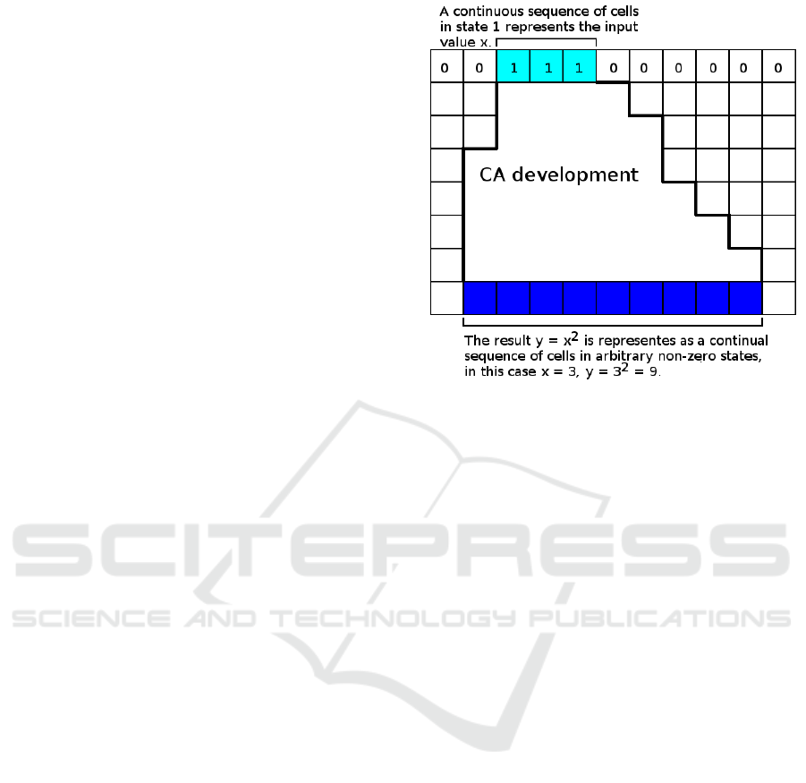
Figure 1: Illustration of encoding integer values in a 1D

ccellular automaton. In this example x = 3, y = 9.

However, it is important to note that CAs with suf-

ﬁcient sizes are used in order to avoid affecting the

development by the ﬁnite number of cells.

The value of x is encoded in the initial CA state as

a continuoussequence of cells in state 1, whose length

(i.e. the number of cells in state 1) corresponds to x,

the other cells possess state 0. For example, the state

of a 12-cell CA, which encodes x = 3, can appear as

0000011100000. The result y = x

, that will emerge

from the initial state in a ﬁnite number of steps, is

assumed as a stable state in which a continuous se-

quence of cells in non-zero states can be detected, the

length of which equals the value of y, the other cells

are required in state 0. For the aforementioned exam-

ple, the result can appear as 002222222220 or even

023231323200 (there is a sequence of non-zero cells

of length 3

= 9). The concept of representing the in-

put value x and the result y is graphically illustrated

in Figure 1. This is a generalised interpretation based

on the idea presented in (Wolfram, 2002), page 639.

The goal is to discover transition functions for the CA,

that are able to calculate the square of arbitrary num-

ber x > 1.

In order to represent the transition functions for

CAs, the concept of Conditionally Matching Rules

(CMR), originally introduced in (Bidlo and Vasicek,

2013), will be applied. This technique showed as

very promising for designing complex cellular au-

tomata (Bidlo, 2015)(Bidlo, 2016). For the 1D CA

working with 3-cell neighbourhood, a CMR is de-

ﬁned as (cond

)(cond

) → s

Cnew

where cond

⋆

denotes a condition function and s

⋆

Evolution of Generic Square Calculations in Cellular Automata

denotes a state value. Each part (cond

⋆

) on the

left of the arrow is evaluated with respect to the state

of a speciﬁc cell in the neighbourhood (in this case

, c

and c

respectively). In this paper the rela-

tion operators =, 6=, ≥ and ≤ are considered as the

condition functions. A ﬁnite sequence of CMRs rep-

resents a transition function. In order to determine

the new state of a cell, the CMRs are evaluated se-

quentially. If a rule is found in which all conditions

are true (with respect to the states in the cell neigh-

bourhood), s

Cnew

from this rule is the new state of the

central cell. Otherwise the cell state does not change.

For example, consider a transition function that con-

tains a CMR (6= 1)(6= 2)(≤ 1) → 1. Let c

states of cells in a neighbourhood with values 2, 3,0

respectively, and a new state of the central cell ought

to be calculated. According to the aforementioned

rule, c

6= s

is true as 2 6= 1, similarly c

6= s

true (3 6= 2) and c

≤ s

(0 ≤ 1). Therefore, this CMR

is said to match, i.e. s

Cnew

= 1 on its right side will

update the state of the central cell.

Note that the evolved CMRs can be transformed

to the conventional table rules (Bidlo, 2016). In this

work the transformation is performed as follows: (1)

For every possible combination of states c

in cellular neighborhood a new state s

Cnew

is calcu-

lated using the CMR-based transition function. (2) If

6= s

Cnew

(i.e. the cell state ought to be modiﬁed),

then a table rule of the form c

→ s

Cnew

is gen-

erated. Note that the combinations of states not in-

cluded amongst the table rules do not change the state

of the central cell, which is treated implicitly during

the CA simulation. The number of such generated

rules will represent a metrics indicating the complex-

ity of the transition function.

In order to determine the complexity of the tran-

sition function with respect to a speciﬁc square cal-

culation in CA, a set of used rules is created using

the aforementioned principle whereas the combina-

tions of states c

are considered just occuring

during the given square calculation in the CA. There

metrics (together with the number of states and CA

steps) will allow us to compare the solutions obtained

by the evolution and to identify the best results with

respect to their complexity and efﬁciency.

An evolutionary algorithm will be applied to

search for suitable CMR-based transition functions as

described in the following section.

3 EVOLUTIONARY SYSTEM

SETUP

In this paper a custom evolutionary algorithm (EA)

was utilised, which is a result of our long-term exper-

imentation in this area. Note, however, that neither

tuning of the EA nor in-depth analysis of the evolu-

tionary process is a subject of this work. The EA is

based on a simple genetic algorithm (Holland, 1975)

with a tournament selection of base 4 and a custom

mutation operator. Crossover is not used as it has not

shown any improvement in success rate or efﬁciency

of our experiments.

The EA utilises the following ﬁxed-length repre-

sentation of the conditionally matching rules in the

genomes. For the purpose of encoding the condition

functions =, 6=, ≥ and ≤, integer values 0, 1, 2 and

3 will be used respectively. Each part (cond

⋆

)

of the CMR is encoded as a single integer P

⋆

in the

range from 0 to M where M = 4∗ S− 1 (4 is the ﬁxed

number of condition functions considered and S is the

number of cell states) and the part → s

Cnew

is repre-

sented by an integer in the range from 0 to S−1. In or-

der to decode a speciﬁc condition and state value, the

following operations are performed: cond

⋆

= P

⋆

/S,

⋆

= P

⋆

mod S (note that / is the integer division

and mod is the modulo-division). This means that a

CMR (cond

)(cond

) → s

Cnew

can

be represented by 4 integers; if 20 CMRs ought to

be encoded in the genome, then 4∗ 20 = 80 integers

are needed. For example, consider S = 3 for which

M = 4∗ 3− 1 = 11. If a 4-tuple of integers (2 9 11 2)

representing a CMR in the genome ought to be de-

coded, then the integers are processed respectively as:

• cond

= 2/3 = 0 which corresponds to the oper-

ator =, s

= 2 mod 3 = 2,

• cond

= 9/3 = 3 which corresponds to the opera-

tor ≤, s

= 9 mod 3 = 0,

• cond

= 11/3 = 3 which corresponds to the oper-

ator ≤, s

= 11 mod 3 = 2,

• s

Cnew

= 2 is directly represented by the 4th integer.

Therefore, a CMR of the form (= 2)(≤ 0)(≤ 2) → 2

has been decoded.

The following variants of the ﬁtness functions are

treated (note that the input x is set to the middle of the

cellular array):

1. RESULT ANYWHERE (RA-ﬁtness): The ﬁtness

is calculated with respect to any valid arrangement

(position) of the result sequence in the CA. For

example, y = 4 in an 8-cell CA may be rrrr0000,

0rrrr000, 00rrrr00, 000rrrr0 or 0000rrrr, where

r 6= 0 represent the result states that may be gen-

erally different within the result sequence. A par-

tial ﬁtness value is calculated for every possible

arrangement of the result sequence as the sum of

the number of cells in the expected state for the

ECTA 2016 - 8th International Conference on Evolutionary Computation Theory and Applications

given values of x. The ﬁnal ﬁtness is the highest

of the partial ﬁtness values.

2. SYMMETRIC RESULT (SR-ﬁtness): The result

is expected symmetrically with respect to the in-

put. For example, if 0000011100000 corresponds

to initial CA state for x = 3, then the result y = 3

is expected as a speciﬁc CA state 00rrrrrrrrr00

(each r may be represented by any non-zero state).

The ﬁtness is the number of cells in the expected

state.

The ﬁtness evaluation of each genome is performed

by simulating the CA for initial states with the val-

ues of x from 2 to 6. The result of the x

calculation

is inspected after the 99th and 100th step of the CA,

which allows to involve the state stability check into

the evaluation. This approach was chosen on the basis

of the maximal x evaluated during the ﬁtness calcula-

tion and on the basis of the number of steps needed

for the square calculation using the existing solution

(Wolfram, 2002). In particular, the ﬁtness of a fully

working solution evaluated for x from 2 to 6 in a 100-

cell CA is given by F

max

= 5 ∗ 2∗ 100 = 1000 (there

are 5 different values of x for which the result x

is in-

vestigated in 2 successive CA states, each consisting

of 100 cells). The evolved transition functions, satis-

fying the maximal ﬁtness for the given range of x, are

checked for the ability to work in larger CAs for up

to x = 25 For the purposes of this paper, the solutions

which pass the check are considered as generic.

The EA works with a population of 8 genomes ini-

tialised randomly at the beginning of evolution. After

evaluating the genomes, four candidates are selected

randomly, the candidate with the highest ﬁtness be-

comes a parent. An offspring is created by mutating

2 randomly selected integers in the parent. The selec-

tion and mutation continue until a new population of

the same size is created and the evolutionary process

is repeated until 2 million generations are performed.

If a solution with the maximal ﬁtness is found, then

the evolutionary run is considered as successful. If

no such solution is found within the given generation

limit, then the evolutionary run is terminated.

4 EXPERIMENTAL RESULTS

The evolutionary design of CAs for the generic square

calculation has been investigated for the following

settings: the number of states 4, 6, 8 and 10, the tran-

sition functions consisting of 20, 30, 40 and 50 CMRs

and two ways of the ﬁtness calculation described in

Section 3. For each setup, 100 independent evolution-

ary runs have been executed. The success rate and av-

erage number of generations needed to ﬁnd a working

solution were observed with respect to the evolution-

ary process. As regards the parameters of the CA, the

minimal number of rules and steps needed to calculate

the square of x were determined.

4.1 Results for the RA-ﬁtness

For the RA-ﬁtness, the statistical results are sum-

marised in Table 1. The table also contains the total

numbers of generic solutions discovered for the given

state setups and parameters determined for these solu-

tions. For every number of states considered, at least

one generic solution was identiﬁed. For example, a

transition function was discovered for the 4-state CA,

which consists of 36 table rules (transformed from

the CMR representation evolved). This solution can

be optimised to 26 rules (by eliminating the rules

not used during the square calculation) which repre-

sents the simplest CA for generic square calculations

known so far (note that Wolfram’s CA works with 8

states and 51 rules (Wolfram, 2002)). Moreover, for

example, our solution needs 74 steps to calculate 6

whilst Wolfram’s CA needs 112 steps, which also rep-

resents a substantial innovation discovered by the EA.

The CA development corresponding to this solution is

shown in Figure 2.

Another result obtained using the RA-ﬁtness is il-

lustrated by the CA development in Figure 3. In this

case the CA works with 6 states and its transition

function consists of 52 effective rules. The number of

steps needed, for example, to calculate 6

, is 46 (and

compared to 112 steps of Wolframs CA, it is an im-

provement of the CA efﬁciency by more than 50%)

which represents the best CA known so far for this

operation and the best result obtained in this paper.

One more example of evolved CA is shown in

Figure 4. This generic solution was obtained in the

setup with 8-state CA, however, the transition func-

tion works with 6 different states only. There are

49 transition rules, the CA needs 68 steps to calcu-

late 6

. This means that the EA discovered a simpler

solution (regarding the the number of states and ta-

ble rules) which is a part of the solution space of the

8-state CA. Again, this result exhibits generally bet-

ter parameters compared to the known solution from

(Wolfram, 2002). The CA development, that was not

observed in any other solution, is also interesting vi-

sually - as Fig. 4 shows, the CA generates a pattern

with some “dead areas” (cells in state 0) within the

cells that subsequently form the result sequence. The

size of these areas is gradually reduced, which ﬁnally

lead to derive the number of steps after which a stable

state containing the correct result for the given x has

emerged (illustrated by the right part of Figure 4 for

Evolution of Generic Square Calculations in Cellular Automata

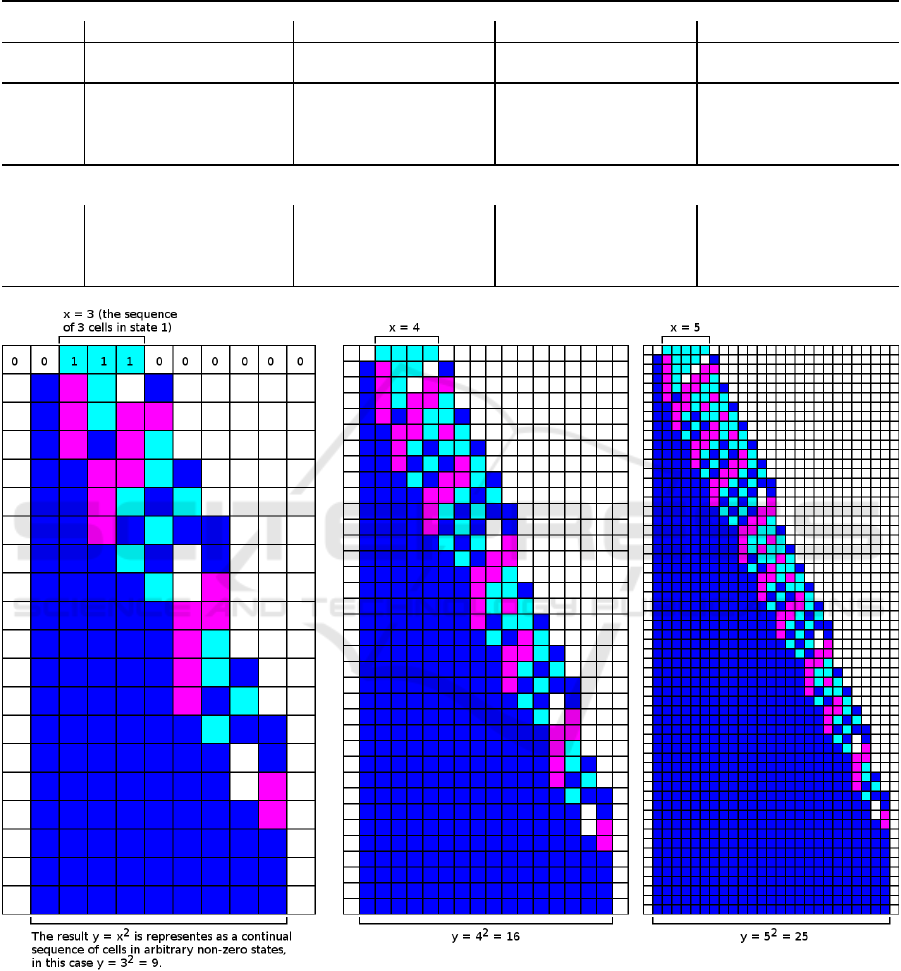
Table 1: Statistics of the evolutionary experiments conducted using the RA-ﬁtness (the upper part of the table) and the

parameters of the generic solutions (in the lower part of the table). The parameters of the best results obtained are marked

bold. Note that # denotes “the number of”, the meaning of “generated rules”, “used rules” and ”steps” of the CA is deﬁned

in Section 2.

the number of states

4 6 8 10

the num. succ. avg. min. min. succ. avg. min. min. succ. avg. min. min. succ. avg. min. min.

of CMRs

rate gen. steps rules rate gen. steps rules rate gen. steps rules rate gen. steps rules

20 3 844364 54 35 30 769440 45 120 45 570939 39 232 35 328210 47 569

30 3 620998 52 36 24 749837 40 120 38 595467 42 340 33 363360 45 663

2 1344286 77 46 19 629122 37 136 30 701612 41 365 29 244566 46 662

50 2 959689 73 43 20 813803 41 134 35 582342 39 348 38 373490 40 762

the number of generic solutions (#generic) obtained for the given number of states

and parameters of the generic solutions: #generated rules/#used rules/#steps for 6

)

#generic,

1 5 6 3

176/52/46, 164/33/87, 435/49/68, 403/51/79, 934/64/56, 835/61/79,

parameters

36/26/74 152/49/78, 185/66/70, 422/39/65, 392/62/76, 916/35/76

175/52/69 423/41/68, 429/94/76

Figure 2: Example of a 4-state squaring CA development for x = 3, 4 and 5 using our most compact transition function. The

rules are: 0 0 1 → 3, 0 1 1 → 2, 0 3 0 → 2, 1 0 0 → 3, 1 0 2 → 2, 1 0 3 → 2, 1 1 0 → 0, 1 1 2 → 2, 1 1 3 → 2, 1 2 1 → 1,

1 3 0 → 1, 1 3 1 → 1, 1 3 2 → 2, 1 3 3 → 0, 2 1 2 → 3, 2 1 3 → 3, 2 2 0 → 1, 2 2 1 → 1, 2 3 1 → 1, 2 3 2 → 2, 3 0 2 → 3,

3 1 0 → 3, 3 1 1 → 3, 3 1 3 → 3, 3 2 0 → 3, 3 2 3 → 3.

x = 8 whereas the CA needs 122 steps to produce the

result).

4.2 Results for the SR-ﬁtness

Table 2 shows the statistics for the SR-ﬁtness together

with the total numbers of generic solutions discovered

ECTA 2016 - 8th International Conference on Evolutionary Computation Theory and Applications

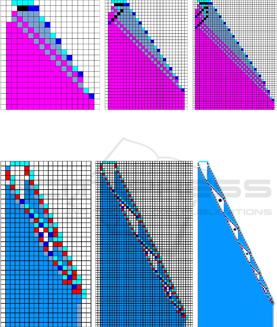
Figure 3: Example of a 6-state CA development for x = 4,5 and 6. This is the fastest CA-based (3-neighbourhood) solution

known so far and the best result obtained in this paper. The rules are: 0 0 4 → 2, 0 0 5 → 2, 0 1 1 → 0, 0 2 3 → 0, 0 2 4 → 4,

0 2 5 → 3, 0 3 2 → 2, 0 3 3 → 0, 0 4 0 → 2, 0 4 2 → 2, 0 5 3 → 0, 0 5 5 → 4, 1 0 0 → 3, 1 1 0 → 3, 1 1 1 → 5, 1 1 4 → 5,

1 4 4 → 5, 2 0 4 → 3, 2 1 0 → 2, 2 2 5 → 5, 2 3 0 → 2, 2 3 4 → 2, 2 4 0 → 2, 2 4 1 → 2, 2 4 2 → 2, 2 4 3 → 2, 2 4 4 → 2,

2 4 5 → 5, 2 5 2 → 2, 2 5 4 → 2, 3 3 0 → 4, 3 4 4 → 2, 4 0 0 → 1, 4 1 0 → 4, 4 1 1 → 4, 4 1 4 → 4, 4 2 0 → 4, 4 2 1 → 4,

4 2 3 → 4, 4 2 4 → 4, 4 3 0 → 4, 4 4 5 → 1, 4 5 1 → 4, 4 5 4 → 4, 4 5 5 → 1, 5 1 1 → 4, 5 1 4 → 4, 5 2 4 → 4, 5 3 3 → 4,

5 5 3 → 4, 5 5 4 → 4, 5 5 5 → 1.

Figure 4: Example of a 6-state squaring CA development (originally designed using 8-state setup) for x = 4,6 and 8. The

development shows a speciﬁc pattern evolved to derive the result of x

, which was not observed in any other solution. The

part on the right shows a complete global behaviour of this CA for x = 8 with some “dead areas” (marked by black spots)

which lead to the correct stable result by progressively reducing the size of these areas (in thic case the result of 8

is achieved

after 122 steps).

for the given state setups and parameters determined

for these solutions. As evident, the success rates are

generally lower compared to the RA-ﬁtness which

is expectable because the SR-ﬁtness allows a single

Evolution of Generic Square Calculations in Cellular Automata

arrangement only of the result sequence in the CA.

Moreover, just two generic CAs have been identiﬁed

out of all the runs executed for this setup. However,

the goal of this experiment was rather to determine

whether solutions of this type ever exist for cellular

automata and evaluate the ability of the EA to ﬁnd

them. As regards both generic solutions, their num-

bers of used rules and CA steps are signiﬁcantly bet-

ter in comparison with Wolfram’s solution (Wolfram,

2002). Speciﬁcally, Wolfram’s solution uses are 51

rules and the calculation of 6

takes 112 steps, whilst

the proposed results use 33, respective 36 rules and

calculate 6

in 71, respective 78 steps. Moreover, one

of them was discovered using a 4-state CA (Wolfram

used 8 states), which belongs to the most compact so-

lutions obtained in this paper and known so far.

Figure 5 shows examples of a CA (identiﬁed as

generic) evolved using the SR-ﬁtness. The transition

function, originally obtained in 8-state CA setup, is

represented by 36 used rules and works with 7 states

only. Although this result cannot be considered as

very efﬁcient (for 6

the CA needs 78 steps), it ex-

hibits one of the most complex emergent process ob-

tained for the square calculation, the result of which is

represented by a non-homogeneousstate. The sample

on the right of Fig. 5 shows a catout of development

for x = 11 in which the global behaviour can be ob-

served. This result demonstrates that the EA can pro-

duce generic solutions to a non-trivial problem even

for a single speciﬁc position of the result sequence re-

quired by the SR-ﬁtness evaluation.

5 DISCUSSION

In most cases of the experimental settings the EA was

able to produce at least one generic solution for the

CA-based square calculation. Despite the 2 million

generation limit, the results from Table 1 and 2 show

that the average number of generations is mostly be-

low 1 million, which indicates a potential of the EA

to efﬁciently explore the search space. In compari-

son with the initial study of this problem proposed

in (Bidlo, 2016), where 200,000 generations were

performed, the signiﬁcant increase of this parameter

herein is important with respect to achieving a rea-

sonable success rate and producing generic solutions

(note that an initial comparison of various ranges for x

evaluated in the ﬁtness was proposed in (Bidlo, 2016),

the result of which was considered in this paper).

As regards the RA-ﬁtness, which can be consid-

ered as the main technique proposed in this paper for

the evolution of cellular automata, a more detailed

analysis was performed with various multi-state CA.

As the results in Table 1 show that the number of

generic solutions increases for the number of states

from 4 to 8, then for 10-state CAs a signiﬁcant re-

duction can be observed. This is probably caused by

the exponential increase of the search space depend-

ing on the number of states. The results indicate that

the 8-state setup represents a very feasible value that

may be considered as sufﬁcient for this kind of prob-

lem (note that 6 generic solutions were obtained for

this setup).

In both sets of experiments with the RA-ﬁtness

and SR-ﬁtness, a phenomenon of a reduction of the

number of states was observed. This is possible due

to the identiﬁcation of just the rules that are needed

for the CA development to calculate the square out

of all the rules generated from the evolved CMR-

based transition function for every valid combination

of states in the cellular neighbourhood. It was deter-

mined that the CAs in some cases do not need all the

available cell states to perform the given operation.

6 CONCLUSIONS

The goal of this paper was the evolutionary design of

uniform cellular automata for the generic square cal-

culation of integer numbers. The representation of the

transition functions for the automata, which utilised

conditionally matching rules, in combination with the

evolutionary algorithm showed that it is possible to

design variousnon-trivialtransition functions for CAs

(published herein for the ﬁrst time) to perform the

generic square calculations in the cellular space us-

ing just local interactions between cells. The analysis

of the results showed a signiﬁcant improvements of

the evolved CA, which overcomes the existing solu-

tion regarding both the complexity of the transition

functions and the number of steps (i.e. speed of the

CA) needed to calculate the given operation. For ex-

ample, a 4-state CA was discovered whose transition

function consists of 26 rules only, which represents

the most compact solution of this problem in the CA

working with a 3-cell neighbourhood known so far.

Another solution presented exhibits a reduction in the

number of CA steps by more than 50% against the

existing approach.

The method applied showed a potential to design

complex CAs that exhibit the given generic behaviour.

Although some different emergent processes in the

resulting CAs were discovered, the detailed analysis

of their behaviour and principles of functioning has

not yet been done (long it was also not the goal of

this paper). Moreover, the evolutionary process it-

self (regarding the details about exploring the solu-

ECTA 2016 - 8th International Conference on Evolutionary Computation Theory and Applications

100

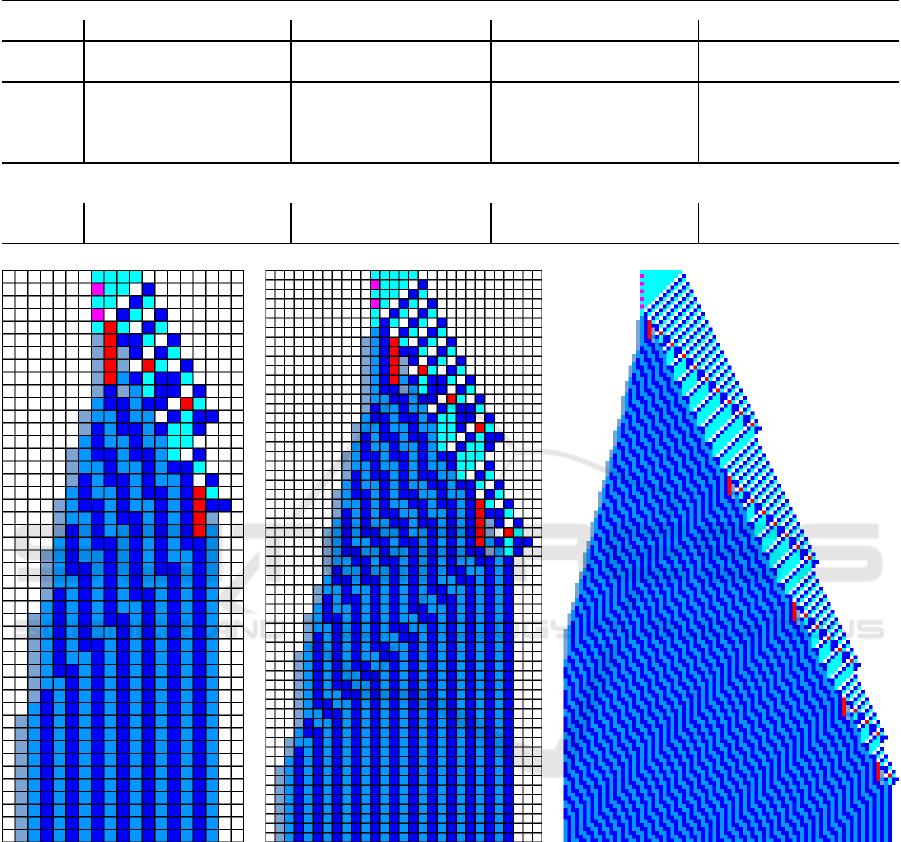
Table 2: Statistics of the evolutionary experiments conducted using the SR-ﬁtness (the upper part of the table) and the param-

eters of the generic solutions (in the lower part of the table). The parameters of the best result obtained are marked bold. Note

that # denotes “the number of”, the meaning of “generated rules”, “used rules” and ”steps” of the CAs is deﬁned in Section 2.

the number of states

4 6 8 10

the num. succ. avg. min. min. succ. avg. min. min. succ. avg. min. min. succ. avg. min. min.

of CMRs

rate gen. steps rules rate gen. steps rules rate gen. steps rules rate gen. steps rules

20 2 634948 71 38 4 734200 38 126 11 982446 34 234 18 855791 53 542

0 - - - 5 905278 48 150 17 934123 51 327 15 910269 35 742

1 1546681 79 45 4 928170 33 147 11 1033059 53 317 15 898314 52 748

0 - - - 3 989039 44 138 12 811686 32 380 17 861850 52 796

the number of generic solutions (#generic) obtained for the given number of states

and parameters of the generic solutions: #generated rules/#used rules/#steps for 6

)

#generic,

1 0 1 0

parameters

38/33/71 234/36/78

Figure 5: Example of a 7-state CA controlled by a transition function evolved using the SR-ﬁtness. A complete development

is shown for x = 4 and 5 (the left and middle sample respectively), the part on the right demonstrates a cutout of global

behaviour of the CA for x = 11 .

tion space using the CMR approach and optimal evo-

lutionary setup) still represents a topic with the work

in progress. Therefore these issues are considered in

our future research.

ACKNOWLEDGEMENTS

This work was supported by the Czech science foun-

dation project 14-04197S and by the Ministry of Ed-

ucation, Youth and Sports of the Czech Republic

from the National Programme of Sustainability (NPU

II); project IT4Innovations excellence in science -

LQ1602.

REFERENCES

Berlekamp, E. R., Conway, J. H., and Guy, R. K. (2004).

Winning Ways for Your Mathematical Plays, 2nd Ed.,

Volume 4. A K Peters/CRC Press.

Bidlo, M. (2015). Investigation of replicating tiles in cel-

Evolution of Generic Square Calculations in Cellular Automata

101

lular automata designed by evolution using condition-

ally matching rules. In 2015 IEEE International Con-

ference on Evolvable Systems (ICES), Proceedings of

the 2015 IEEE Symposium Series on Computational

Intelligence (SSCI), pages 1506–1513. IEEE Compu-

tational Intelligence Society.

Bidlo, M. (2016). On routine evolution of com-

plex cellular automata. IEEE Transactions on

Evolutionary Computation, PP(99):1–13, URL:

http://ieeexplore.ieee.org/stamp/stamp.jsp?tp=

&arnumber=7377086&isnumber=4358751.

Bidlo, M. and Vasicek, Z. (2013). Evolution of cellular au-

tomata with conditionally matching rules. In 2013

IEEE Congress on Evolutionary Computation (CEC

2013), pages 1178–1185. IEEE Computer Society.

Codd, E. F. (1968). Cellular Automata. Academic Press,

New York.

Durand, B. and Rka, Z. (1999). The game of life: Uni-

versality revisited. In Mathematics and Its Applica-

tions, Volume 460 Cellular Automata, pages 51–74.

Springer Netherlands.

Holland, J. H. (1975). Adaptation in Natural and Artiﬁcial

Systems. University of Michigan Press, Ann Arbor.

Ilachinski, A. (2001). Cellular Automata: A Discrete Uni-

verse. World Scientiﬁc.

Jean-Yves Perrier, Moshe Sipper, J. Z. (1996). Toward a

viable, self-reproducing universal computer. Physica

D, 97(4):335–352.

Lindgren, K. and Nordahl, M. G. (1990). Universal com-

putation in simple one-dimensional cellular automata.

Complex Systems, 4(3):299–318.

Mardiris, V., Sirakoulis, G., and Karafyllidis, I. (2015). Au-

tomated design architecture for 1-d cellular automata

using quantum cellular automata. Computers, IEEE

Transactions on, 64(9):2476–2489.

Ninagawa, S. (2013). Solving the parity problem with rule

60 in array size of the power of two. Journal of Cel-

lular Automata, 8(3–4):189–203.

Rendell, P. (2011). A universal turing machine in con-

way’s game of life. In 2011 International Confer-

ence on High Performance Computing and Simulation

(HPCS), pages 764–772.

Rendell, P. (2013). A fully universal turing machine in Con-

way’s game of life. Journal of Cellular Automata,

9(1–2):19–358.

Sahoo, S., Choudhury, P. P., Pal, A., and Nayak, B. K.

(2014). Solutions on 1-d and 2-d density classiﬁca-

tion problem using programmable cellular automata.

Journal of Cellular Automata, 9(1):59–88.

Sahu, S., Oono, H., Ghosh, S., Bandyopadhyay, A., Fu-

jita, D., Peper, F., Isokawa, T., and Pati, R. (2010).

Molecular implementations of cellular automata. In

Cellular Automata for Research and Industry, Lecture

Notes in Computer Science, Vol. 6350, pages 650–

659. Springer.

Sipper, M. (1995). Quasi-uniform computation-universal

cellular cutomata. In Advances in Artiﬁcial Life,

ECAL 1995, Lecture Notes in Computer Science, Vol.

929, pages 544–554. Springer Berlin Heidelberg.

Sridharan, K. and Pudi, V. (2015). Design of Arithmetic Cir-

cuits in Quantum Dot Cellular Automata Nanotech-

nology. Springer International Publishing Switzer-

land.

Stefano, G. D. and Navarra, A. (2012). Scintillae: How to

approach computing systems by means of cellular au-

tomata. In Cellular Automata for Research and Indus-

try, Lecture Notes in Computer Science, Vol. 7495,

pages 534–543. Springer.

Tempesti, G. (1995). A new self-reproducing cellular au-

tomaton capable of construction and computation. In

Advances in Artiﬁcial Life, Proc. 3rd European Con-

ference on Artiﬁcial Life, Lecture Notes in Artiﬁcial

Intelligence, Vol. 929, pages 555–563. Springer.

von Neumann, J. (1966). The Theory of Self-Reproducing

Automata. A. W. Burks (ed.), University of Illinois

Press.

Wolfram, S. (2002). A New Kind of Science. Wolfram Me-

dia, Champaign IL.

Yuns, J.-B. (2010). Achieving universal computations

on one-dimensional cellular automata. In Cellular

Automata for Research and Industry, Lecture Notes

in Computer Science Volume 6350, pages 660–669.

Springer.

ECTA 2016 - 8th International Conference on Evolutionary Computation Theory and Applications

102