An Optimal Trajectory Planner for a Robotic Batting Task: The Table

Tennis Example

Diana Serra

, Aykut C. Satici

, Fabio Ruggiero

, Vincenzo Lippiello

and Bruno Siciliano

Department of Electrical Engineering and Information Technology, University of Naples Federico II,

Via Claudio 21, 80125, Naples, Italy

Electrical Engineering and Computer Science, Massachusetts Institute of Technology,

32 Vassar Street, Cambridge, Massachusetts, U.S.A.

Keywords:

Optimal Trajectory Planning, Table Tennis Robot, Nonprehensile Manipulation.

Abstract:

This paper presents an optimal trajectory planner for a robotic batting task . The speciﬁc case of a table tennis

game performed by a robot is considered. Given an estimation of the trajectory of the ball during the free ﬂight,

the method addresses the determination of the paddle conﬁguration (pose and velocity) to return the ball at a

desired position with a desired spin. The implemented algorithm takes into account the hybrid dynamic model

of the ball in free ﬂight as well as the state transition at the impact (the reset map). An optimal trajectory that

minimizes the acceleration functional is generated for the paddle to reach the desired impact position, velocity

and orientation. Simulations of different case studies further bolster the approach along with a comparison

with state-of-the-art methods.

1 INTRODUCTION

Interest in robotic manipulation without grasping the

objects, i.e., nonprehensile manipulation, is recently

rising. The presence of unilateral constraints in-

creases the complexity in planning and control the

robot that has to dynamically drive the manipulated

object from the initial to the desired conﬁguration.

Nevertheless, as highlighted by (Lynch and Mason,

1999), nonprehensile manipulation allows controlling

extra degrees of freedom. The workspace is thus

increased since the manipulated object can physi-

cally overcome the kinematic limitations of the end-

effector by continuously breaking and creating con-

tacts with the robot. Therefore, a nonprehensile ma-

nipulation task is in general complex, skillful and dex-

terous. Normally, it can be undertaken by splitting

the complex task in many simpler subtasks, usually

called primitives, such as rolling, sliding, throwing,

catching, pushing and batting. The latter is the one

addressed in this paper. Batting combines catching

and throwing in a single collision: a practical exam-

ple is given by the table tennis game. Such a task

requires so high velocities and precision that robotic

companies take it as an example to display the high

performances of their products. For instance, Kuka

has chosen the table tennis game to promote its wares

in a thrilling commercial spot (Kuka, 2014), showing

the potential abilities of robots. The Omron automa-

tion company has also broadcast a video showing its

parallel Delta robot playing table tennis and coaching

humans at CEATEC Japan 2015 exhibition, (Omron,

2015).

The robotic batting task can be tackled with differ-

ent approaches. From the artiﬁcial intelligence point

of view, for instance, the aim is to improve the per-

formance of the robot through experience, while also

dealing with temporal issues; from the planning and

control points of view, instead, accurate models are

researched and investigated for autonomous and fast

motion execution; from the perception side, ﬁnally,

fast and reliable measurements are requested. This

paper is focused on planning and control aspects, in-

herently considering the hybrid nature of the system

and real-time constraints.

Generally, a robotic system for a batting task (e.g.,

table tennis) should be provided by: a vision system

to track the motion of the ball, a method to estimate

the trajectory of the ball in free ﬂight and its spin,

a decision system to choose the paddle conﬁguration

to direct the ball towards the desired position on the

opposite court, and a trajectory planner for the motion

of the paddle.

The scope of this paper is to provide an optimal

trajectory planner for the paddle to return the ball to

the opposite court at a desired position with an im-

Serra, D., Satici, A., Ruggiero, F., Lippiello, V. and Siciliano, B.

An Optimal Trajectory Planner for a Robotic Batting Task: The Table Tennis Example.

DOI: 10.5220/0005982000900101

In Proceedings of the 13th International Conference on Informatics in Control, Automation and Robotics (ICINCO 2016) - Volume 2, pages 90-101

ISBN: 978-989-758-198-4

posed spin. At the same time, an improvement of

the decision system proposed by (Liu et al., 2012) to

choose the conﬁguration of the paddle at the impact

time is here described. The proposed algorithm con-

sists of two main phases: the hybrid model solution,

computing the state of the paddle at the impact time

such that the control objective is satisﬁed, and the tra-

jectory optimization in SE(3), providing the angular

and linear trajectory of the paddle up to the impact

time.

The novelties introduced by this manuscript are

twofold.

• Firstly, in comparison to the state-of-the-art, the

proposed method improves the control accuracy

by considering a full aerodynamic model of the

ball, and taking into account drag and lift forces.

The computation time of the algorithm is also

fast enough to guarantee it can suitably be imple-

mented in real-time.

• Secondly, rigorous methods from calculus on

manifolds are borrowed to generate an optimal

trajectory on SE(3) for the paddle to strike the ball

at the impact time.

2 RELATED WORK

(Andersson, 1989a) describes a tracking system and

a trajectory generation for a table tennis robot player.

The method uses ﬁfth-order polynomials to generate

a trajectory for the paddle intercepting the ball. The

architecture is designed so that the task level control

can monitor the torques of the robot during the move-

ments of the arm, and also adjust the trajectory while

the ball is in free ﬂight. (Andersson, 1989b) shows

how the processing time of a stereo vision system

should be taken into account when it is applied to a

quickly changing operating environment. A table ten-

nis robot player prototype equipped with two levels

control system is described by (Acosta et al., 2003).

The objective of the lower level is to move the cen-

ter of the paddle to the right position to intercept the

ball. The high-level control deﬁnes instead the game

strategy. This is done by orienting the paddle to return

the ball to the desired position on the table. The pro-

totype is capable of returning balls with a good suc-

cess rate when their velocity is below 5 m/s and under

small spin effects. A high-speed trajectory planner is

described by (Senoo et al., 2006) and it is applied to

the batting task. The authors also consider the robot

dynamic model within their framework, and they rely

upon a 1kHz high-speed vision system. Nevertheless,

they do not go into details about the controller com-

putational efforts, and they use a simpliﬁed version

of the reset map in which the spin of the ball after

the impact is not considered. Spin is indeed relevant

for the table tennis game. Moreover, the trajectory

planner they use is based on polynomial primitives,

which has been demonstrated to demand high joint

accelerations. (Nakashima et al., 2010) show how to

obtain the linear and angular ball trajectory informa-

tion from the visual sensors. On the other hand, (Liu

et al., 2012) propose a control method for returning a

table tennis ball to a desired position with a desired

spin. The method determines the state of the paddle

employing the hybrid dynamic model of the ball in

free ﬂight as well as the state transition at the impact.

In order to determine the control action, an approx-

imated aerodynamic model is considered, providing

a satisfactory but less accurate results. (Nakashima

et al., 2014) follow up the work of (Liu et al., 2012) by

focusing on the nonlinear aerodynamics solution. A

ﬁnite difference method and a linearization of the dis-

cretized model are employed to solve the two bound-

ary values problem so as to reduce the computational

time. However, they present fewer case studies than

(Liu et al., 2012), while the obtained results are not

so easy to reproduce due to a lack of implementation

details.

The artiﬁcial intelligence research community is

applying many learning techniques to the robotic ta-

ble tennis task. (Matsushima et al., 2005) describe

an approach to perform the table tennis task based

on learning. Some impressive table tennis games be-

tween two humanoid robots are performed using the

adaptive trajectory prediction developed by (Zhang

et al., 2012). This model involves an ofﬂine train-

ing of the parameters on the base of the recorded state

of the ball. Afterwards, the model parameters are on-

line adapted for estimation and prediction processes.

Other approaches reproduce the movements learned

from human demonstrations. (M

ulling et al., 2010)

pursue trajectory generation for the robotic table ten-

nis task from a biomimetic point of view. In the ap-

proach introduced by (M

ulling et al., 2013), the robot

ﬁrst learns a set of elementary table tennis hitting

movements from a human table tennis teacher, and

then generalizes those movements in a wider range

of situations using a mixture of motor primitives ap-

proach. (Huang et al., 2013) propose an active learn-

ing approach where the initial parameters related to

the paddle are computed through a locally weighted

regression method. A simpliﬁed hitting scenario task

is implemented by (Oubbati et al., 2013), where a

robot arm hits a ball rolling on an inclined plane

placed in front of the robot. The authors propose a

model that autonomously generates and organizes se-

quences of timed actions. The timing of the move-

An Optimal Trajectory Planner for a Robotic Batting Task: The Table Tennis Example

ments is controlled by nonlinear oscillators. Their ac-

tivation and deactivation are coordinated by a hierar-

chical neural dynamic architecture. (Yanlong et al.,

2015) ﬁnd optimal striking points for a table tennis

robot. The choice is based on a reward function,

measuring how well the trajectory of the ball and the

movement of the paddle coincide. Given the striking

point, a stochastic policy over the reward is derived to

evaluate prospective striking points sampled from the

predicted rebound trajectory. In that approach, the re-

sulting learning method takes into account the amount

of experience data and its conﬁdence.

Recently, researchers of aerial robotics have also

been interested in the batting problem. A control ap-

proach to juggle a ball between either a human and

a quadrotor or two quadrotors is showed by (M

uller

et al., 2011). (Silva et al., 2015) tackle the task of

hitting a table tennis ball with a commercial drone.

The ball tracking relies only upon the onboard cam-

era and not upon an external motion capture system.

The estimation of the hitting point is performed us-

ing a variation of regularized kernel regression, where

samples are weighted according to their relevance to

the task. The decision phase determines the hitting

motion from a set of primitives learned from human

demonstrations. Finally, (Wei et al., 2015) present

a trajectory tracking control strategy for a ball jug-

gling task on a quadrotor, based on the subspace sta-

bilization approach. An optimal trajectory generation

method is adopted to obtain a dynamically feasible,

minimum jerk trajectory.

3 HYBRID DYNAMIC

MODELING

The hybrid dynamics of the ball consists of the free

ﬂight aerodynamics and the impact reset map. The

former is modeled through Newton’s equations of

motion, while the latter is a reset of the state, updated

according to the impact detection. In order to ana-

lytically model the ball dynamics, the work by (Liu

et al., 2012) is considered. That work is supported

by simulations and experiments in several case stud-

ies and follows up a deep study on the hybrid dynamic

modeling of the table tennis game, (Nakashima et al.,

2010). On the other hand, a ﬁrst-order dynamics for

the paddle is here introduced, assuming that it is pos-

sible to directly control its velocity.

It is assumed that a point contact occurs between

the ball and the paddle during the impact. Moreover,

as long as the paddle is made of rubber, the rebound

in the direction normal to the paddle’s plane does not

affect the motion of the ball in the other directions.

Figure 1: Ball and paddle coordinate systems.

Finally, since the mass of the paddle is usually bigger

than the mass of the ball, only the velocity of the ball

is considered to be affected by the impact.

According to Figure 1, let Σ

be the ﬁxed world

frame, Σ

be the frame placed at the center of the

paddle, where the z-axis is the outward normal, and

be the frame placed at the center of the ball. Let





∈ R

be the position of the

ball, v





∈ R

be the velocity of

the ball, ω





∈ R

be the spin

of the ball, assumed constant during the free ﬂight,





∈ R

be the position of the

paddle, v





∈ R

be the velocity

of the paddle, ω





∈ R

be the

angular velocity of the paddle, all expressed in Σ

Finally, let R

∈ SO(3) be the rotation matrix of Σ

with respect to Σ

The continuous ball and paddle dynamics are

given by

= v

, (1a)

= −g − k

||v

+ k

S(ω

, (1b)

= v

, (1c)

= R

S(ω

), (1d)

where g =



0 0 g



is the gravity acceleration,

||·|| is the Euclidean norm, S(·) ∈ R

3×3

is the skew-

symmetric matrix operator. k

and k

are drag and lift

parameters, respectively, and they are typically mod-

elled as

= k

,ω

) =

ρπr

+ b

f (v

,ω

))

, (2a)

= k

,ω

) =

ρ4πr

+ b

f (v

,ω

))

, (2b)

with

f (v

,ω

) =

1 +

)ω

−v

)

. (3)

The meaning of other parameters, like ρ, r, a

, a

, b

, and their numerical values employed in sim-

ulations are depicted in Section 6, Table 1, where a

ICINCO 2016 - 13th International Conference on Informatics in Control, Automation and Robotics

standard table tennis ball and a rubber paddle have

been considered.

Since the paddle can modify the ball velocity only

at the impact time, the control action, represented by

the paddle linear and angular velocities, enters the ball

dynamics through the reset map. Assuming that the

superscripts − and + represent the state before and

after the impact time, respectively, the rebound equa-

tions are given by

= v

+ R

−

− v

) + R

vω

−

(4a)

= R

ωv

−

− v

) + R

ωω

−

, (4b)

where the matrices of rebound coefﬁcients are deﬁned

= diag(1 − e

,1 − e

),A

vω

= −e

rS(e

(5)

ωv

= e

rS(e

),A

ωω

= diag(1 − e

,1 − e

,1),

where e

∈ R

is the unit vector along the i

-axis, i =

{1,2,3}, while e

and e

are described in Section 6,

Table 1.

Notice that (1b) takes into account the spin of the

ball: the magnitude of the drag and lift forces and

their coefﬁcients change according to the spin, inﬂu-

encing the trajectory of the ball. The values of the

components of ω

determine the kind of the spin,

namely: backspin, if ω

> 0; topspin, if ω

< 0;

and sidespin, if ω

> 0. The effect of the spin of the

ball in a table tennis game is not negligible and makes

a difference between a serious table tennis player and

a novice one. Serious players use spin on both their

serves and rallying shots to control the ball and to

force errors from their opponents.

4 BATTING PROBLEM

SOLUTION

In order to accomplish the task of hitting the table ten-

nis ball and directing it to a desired position on the

opposite court with a desired spin, the paddle must

intercept the ball with a certain orientation and ve-

locity. These inputs are computed employing the dy-

namics of the ball in different steps. Firstly, the im-

pact position p





∈ R

and ve-

locity v

−

are predicted by assigning the impact time t

and the initial position p





∈ R

and velocity v





∈ R

of the ball

produced by the opponent’s hit. This step is accom-

plished solving forward the model (1a)-(1b). Once

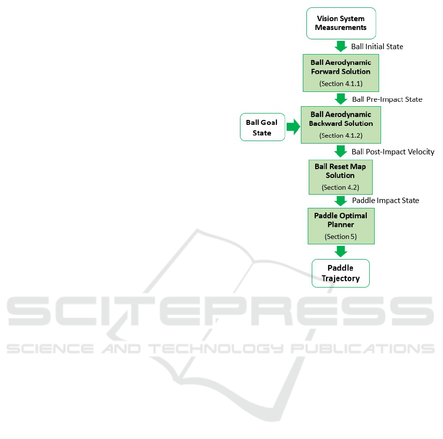
Figure 2: Scheme of the steps to generate the paddle trajec-

tory.

the impact position is predicted, assigning the de-

sired position of the ball on the opposite court p





∈ R

, the desired arrival time t

and the desired spin of the ball after the impact,

∈ R

, solving backward (1a)-(1b) yields the re-

quired velocity of the ball after the impact v

∈ R

Afterwards, the orientation R

and velocity v

of the

paddle at the impact time may be retrieved, through

the reset map (4), once the spin and velocity of the

ball before and after the impact are assigned. Lastly,

the paddle desired impact conﬁguration is the input

of the optimal trajectory planner described in the next

section. A scheme of the steps required to generate a

suitable paddle trajectory is showed in Figure 2.

4.1 Aerodynamic Model Solution

In order to predict the impact state of the ball and

to compute the post-impact velocity of the ball such

that it reaches the goal, the equations (1a) and (1b) of

the aerodynamic model are employed. However, this

model is nonlinear and coupled, thus an analytic so-

lution does not exist. In the literature (Acosta et al.,

2003), (M

uller et al., 2011) and others have consid-

ered a linearized model, or a simpliﬁed one for control

An Optimal Trajectory Planner for a Robotic Batting Task: The Table Tennis Example

purposes to reduce the computations.

The following simpliﬁed model of (1a)-(1b) is em-

ployed by (Liu et al., 2012) since it has an analytic

solution

˙v

= −c

, ˙p

= v

, (6a)

˙v

= −c

, ˙p

= v

, (6b)

˙v

= −g, ˙p

= v

, (6c)

where c

is a constant drag parameter. In this paper,

instead, a numerical solver suitable for real-time pro-

cess is employed to solve the full aerodynamic model.

The proposed algorithm consists in the two minimiza-

tion problems shown below.

4.1.1 Aerodynamic Forward Solution

The ﬁrst problem has the aim to predict the impact

position and velocity of the ball. By assigning the im-

pact time, the ball impact state is predicted according

to the initial position and velocity of the ball produced

by the opponent’s hit. In detail, the algorithm solves

the following minimization problem

min

−







−







, (7)

where p

and v

−

are the optimizing variables,

−

) and

−

) are the position and

the velocity of the ball at the initial time, respec-

tively, numerically obtained by backward integrat-

ing (1a) and (1b) starting from the optimization vari-

ables p

−

at time t

. In practice, the minimiza-

tion problem (7) is solved through the Levembert-

Marquardt’s algorithm that is well suited for real-

time computations according to (Lippiello and Rug-

giero, 2012) and (Cigliano et al., 2015). To speed

up the convergence of the nonlinear estimation algo-

rithm (7), the initial guess for p

and v

−

is calculated

analytically from (6). The work by (Liu et al., 2012)

assumes instead that the impact position of the pad-

dle with the ball is a-priori known. Such assumption

is quite restrictive: hence, here the determination of

such impact position is addressed at run-time.

4.1.2 Aerodynamic Backward Solution

In order to compute the velocity v

of the ball after

the impact such that it reaches the goal position p

at the time t

, the following minimization problem is

solved

min

) − p

, (8)

where v

is the optimization variable and

) is

the position of the ball at time t

numerically obtained

by forward integrating (1a) and (1b) starting from p

at t

computed in Section 4.1.1. The result of the min-

imization problem is the value of the velocity of the

ball after impact so that it reaches the desired posi-

tion on the opposite court at t

as close as possible.

The initial guess for v

is calculated analytically from

(6). This choice of the initial condition, together with

the use of the complete aerodynamic model (1a)-(1b)

in (8) to compute

), guarantees that the value

of v

found by solving (8) is more precise than the

one provided by (6), since the latter employs only a

simpliﬁed model.

4.2 Reset Map Solution

Given the pre-impact velocity of the ball v

−

as in

Section 4.1.1, and the post-impact one v

as in Sec-

tion 4.1.2, the paddle conﬁguration can be now com-

puted. Consider the YX-Euler angles (θ,φ) as a para-

metric representation of the orientation of the paddle,

with φ ∈ [−π/2,π/2] and θ ∈ [0,π], and deﬁne

v =



˜v



= v

−v

−

and

ω =





− ω

−

. The velocity and orientation of the paddle

at the impact time are respectively computed through

= v

−

+ R

− A

)

−1

v − A

vω

−

), (9a)

= R

(θ)R

(φ), (9b)

where I

∈ R

3×3

is the identity matrix, R

(·) ∈ SO(3)

is the elementary rotation matrix with i = {X,Y }, rep-

resenting the rotation of an angle around the i-axis,

and θ,φ are such that

˜v

cosφ sinθ − ˜v

cosφ cosθ =

, (10a)

asin

φ − 2b sinφ + c = 0, (10b)

where a = e

v||

, b = e

ω, c = (e

)||

ω||

−e

v||

, and e

= e

r/e

. Notice that the

ball motions have to satisfy the proposition given by

(Liu et al., 2012) (Proposition 1, Section III-A) to

guarantee the existence of a solution.

5 OPTIMAL PADDLE

TRAJECTORY PLANNING

In this section, the problem of generating an optimal

trajectory for the end-effector of the paddle is tackled.

The control design procedure from the previous sec-

tion provides a desired pose and velocity of the pad-

dle and corresponding desired time instant at which to

achieve these. There are many different paths that the

paddle can take to fulﬁll these requirements. A more

judicious method would be to plan this path such that

ICINCO 2016 - 13th International Conference on Informatics in Control, Automation and Robotics

a certain objective function is optimized. Differential

geometry offers a way to extend the notion of differ-

entiation from Euclidean space to an arbitrary mani-

fold. Primarily, a short background about differential

geometry is here reported, consequently, the theory

about the minimum acceleration planner for the pad-

dle is described.

5.1 Differential Geometry Background

In this context, trajectories for which it is possible to

specify the initial and ﬁnal position and velocity of the

motion are of interest. Note that, the motion may be

speciﬁed in either the joint space, which is a torus, or

the task space, which is the special Euclidean group

of three-dimensions over the reals. At this stage, it

is assumed that the path is generated on an arbitrary

Riemannian manifold M (do Carmo, 1992). Let γ :

(a,b) −→ M be the path, and

⟪

·, ·

⟫

be the metric on

M. Let f : (−ε,ε) × (a,b) −→ M be a proper variation

of γ; that is, it satisﬁes

f (0,t) = γ(t), ∀t ∈ (a,b)

f (s,a) = γ(a), and f (s,b) = γ(b)

Two vector ﬁelds are relevant along the path γ. The

ﬁrst one is called the variation ﬁeld and is deﬁned by

γ(s)

∂ f (s,t)

∂s

d f

(s)

The second vector ﬁeld of importance is the velocity

vector ﬁeld of γ, given by

γ(s)

dγ(t)

∂ f (s,t)

∂t

d f

(t)

In order to perform calculus on the curves of this Rie-

mannian manifold, the Levi-Civita connection ∇ is in-

troduced. Given a curve γ(t) and a connection, there

exists a covariant derivative, which is denoted by

The Levi-Civita connection satisﬁes the following

compatibility and symmetry conditions, presented in

this order:

(11a)

⟪U,W ⟫ = ⟪

,W ⟫ + ⟪U,

⟫

(11b)∇

Y − ∇

X = [X ,Y ]

for any vector ﬁelds U and W , along the differentiable

curve γ, and any vector ﬁeld X,Y ∈ X(M).

The curvature R of a Riemannian manifold M is

a correspondence that associates to every pair X,Y ∈

X(M) a mapping R(X,Y ) : X(M) −→ X(M) given by

R(X,Y )Z = ∇

∇

Z − ∇

∇

Z + ∇

[X,Y ]

where Z ∈ X(M). Some of the properties of the cur-

vature that are going to be used are

∂t

∂s

X −

∂s

∂t

X = R



∂ f

∂s

∂ f

∂t



hR(X,Y )Z, T i = hR(Z,Y )X,Y i.

5.2 Minimum Acceleration Planning

In this work, the acceleration functional in SE(3) is

minimized by following theory developed in (Zefran

et al., 1998). The acceleration functional to be mini-

mized by the choice of the path to be followed by the

paddle is

(12)J =

∇

V,∇

dt,

where [t

] is the time interval over which the trajec-

tory is planned, V = (ω

) ∈ se(3) is the velocity

of the paddle along a particular path, and ∇ denotes

the Levi-Civita afﬁne connection derived from a par-

ticular choice of metric on SE(3). This latter object

allows one to perform differentiation along curves on

any smooth manifold. In particular, in (12), it is used

to express the inner product of the acceleration of a

particular path with itself, which may also be identi-

ﬁed by the squared norm of the acceleration of this

path at a particular point. If the metric on SE(3) is

taken in the form

W =



αI

0 βI



where α,β > 0 so that for T

∈ se(3), then

⟪T

⟫ = t

with t

and t

the 6 × 1 compo-

nents of T

and T

, then the Levi-Civita connection

can be computed to be

∇

Y =



× ω

+ ω

× v



where ω

and ω

are the angular components and v

and v

are the linear components of the rigid body

velocities X ∈ se(3) and Y ∈ se(3), respectively.

Equating the ﬁrst variation of the cost func-

tional (12) to zero provides necessary conditions for

the path to be a minimizer of the acceleration func-

tional. This necessary condition is a fourth order

boundary problem given by

(13)∇

∇

V + R (V,∇

V)V = 0,

where R is the curvature tensor associated with the

Levi-Civita afﬁne connection (do Carmo, 1992). This

condition can be written down in terms of the angular

and linear velocity components of the paddle as

(14a)ω

(3)

+ ω

= 0,

(14b)p

(4)

= 0,

where (·)

(n)

denotes the n

derivative of (·). These or-

dinary differential equations turn into a well-deﬁned

boundary value problem with the addition of the

An Optimal Trajectory Planner for a Robotic Batting Task: The Table Tennis Example

boundary conditions. For the differential equa-

tions (14a) governing the optimal rotational path, the

boundary conditions are

(15a)R

) = R

) = ω

(15b)R

) = R

, ω

) = ω

where R

and ω

are the initial orientation and angu-

lar velocity of the paddle, respectively. Similarly for

the differential equations (14b) governing the optimal

translational path of the paddle, the boundary condi-

tions are

(16a)p

) = p

) = v

(16b)p

) = p

) = v

In practice, the optimal translational motion of the

paddle is found by merely solving a small scale linear

system of equations obtained by (14b) and (16). As

a result, it may be performed very fast. On the other

hand, in order to determine the rotary motion of the

paddle, a boundary value problem needs to be solved.

The boundary value problem is time invariant and non

linear, but the forcing function (14a) is hardly compli-

cated. In Section 6, the computational burden of the

proposed optimal paddle trajectory planner is deeply

analysed.

6 SIMULATIONS

This section shows the results obtained in simulation.

Section 6.1 shows an exemplar simulation of the pro-

posed algorithm (see Figure 2). The comparative case

studies in Section 6.2 show instead the results of the

comparison between the proposed solution to com-

pute the ball post-impact velocity (see Section 4.1.2)

and the one used in (Liu et al., 2012). Lastly, in Sec-

tion 6.3 the optimal planner simulations are focused

on the paddle motion to highlight the properties of

the planned trajectories.

The model parameters considered to simulate the

physical system (1) and (4) are listed in Table 1. A

procedure to identify the aerodynamic and rebound

parameters is described by (Nonomura et al., 2010).

The simulations described below are implemented

in the Matlab environment: the ode45 solver, with

the events option, is used for the dynamic model;

the lsqcurve f it function, based on the Levembert-

Marquardt’s algorithm, is employed to ﬁnd the aero-

dynamic forward and backward solutions; the bvp4c

function is used for the minimum acceleration plan-

ner.

Table 1: Dynamic parameters.

r Ball radius 2e-2 m

Paddle radius 1.5e-1 m

m Ball mass 2.7e-3 kg

ρ Air density (25

◦

C) 1.184 kg/m

g Gravity constant 9.81 m/s

Velocity rebound coefﬁcient 6.15e-1

Spin rebound coefﬁcient 2.57e3

Linear rebound coefﬁcient 7.3e-1

Drag coefﬁcient 5.05e-1

Drag coefﬁcient 6.5e-2

Lift coefﬁcient 9.4e-2

Lift coefﬁcient -2.6e-2

Simpliﬁed drag coefﬁcient 5.4e-1

6.1 Batting Task Simulation

In this case study the proposed algorithm, depicted in

Figure 2, is simulated. Then, supposing to have at dis-

position the estimated trajectory of the ball from the

visual system and the desired ﬁnal conﬁguration of

the ball, it is possible to compute the optimal paddle

trajectory to achieve the batting task through the two

minimization problems (7) and (8), and the solution

of (9) and (14).

Therefore, the visual measurement system is as-

sumed to provide the initial position, linear and an-

gular velocity produced by the opponent’s hit, re-

spectively correspondent to p



1.2 0.7 0.9





−3 0.2 1.5



m/s and ω

−



0,150, 0



. The

impact time is ﬁxed to t

= 0.5 s and the desired ﬁnal

position of the ball on the opposite court is assigned

as p



1.9 0.8 0.02



m. The desired ﬂight time

and post-impact ball spin are assumed to be respec-

tively t

= 0.6 s and



,ω





−100,0



rad/s.

The third component of the desired post-impact spin

of the ball, ω

, is computed from the equation

= 0. It is remarkable that, since the goal is

achieved when the ball hits the table on the opposite

court, the ﬁnal goal time is evaluated when the third

component of the position vector of the ball is equal

to the radius of the ball.

In this case study, the aerodynamic forward solu-

tion of (7) is p



−0.1394 0.7892 0.4820



and v

−



−2.4156 0.1570 −2.9788



m/s, the

aerodynamic backward solution of (8) is v



4.0516 0.0214 2.0984



m/s, while the solution of

reset map (9) is





0.8614 0.0054 0.5080

0 0.9999 −0.0106

−0.5080 0.0092 0.8613





and v



1.4388 0.0220 −0.1131



m/s. The

ICINCO 2016 - 13th International Conference on Informatics in Control, Automation and Robotics

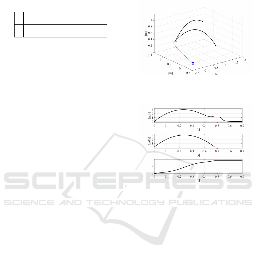
Table 2: Ball pre-impact conﬁguration.

−

[m/s]

−

[rad/s]



−2.5,0,0.1

 

0,150,0





−4.5,0,0.3

 

0,−150,0





−2.75,−0.8,−0.5

 

0,−50,150



optimal trajectory is consequently planned solv-

ing (14).

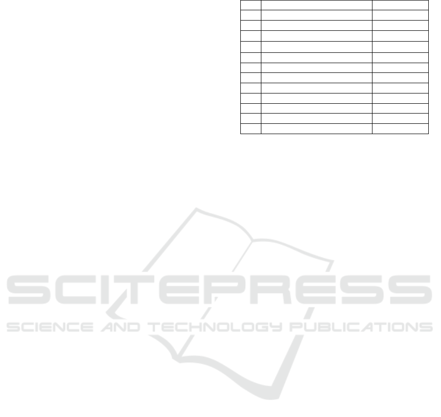
The time histories given by the simulation of this

case study are depicted in Figure 3. In particular, the

3D trajectories of both the ball and the paddle are rep-

resented in Figure 3(a). The solid line represents the

motion of the ball, while the trajectory for the paddle

is depicted by a dashed line. The blue cross represents

the ﬁnal desired position of the ball p

, while the blue

circle is the initial position of the paddle p

. Assum-

ing that ∆t

is the difference between the planned and

the actual impact time, ∆p

the Euclidean norm of

the difference between the planned impact position of

the ball and the actual one, ∆t

the difference between

the desired ﬁnal time and the actual one, ∆p

the Eu-

clidean norm of the difference between the desired

position of the ball p

and the actual one. In this case

study, the time and position impact and ﬁnal errors

are respectively ∆t

= 4.5e − 3 s, ∆p

= 1.73e − 2 m,

∆t

= 1.9e − 3 s and ∆p

= 9.4e − 3 m. Therefore,

the average of the errors is acceptably small for a ta-

ble tennis robot.

A video can be found in (Serra et al., 2016) which

shows the simulation of this case study performed in

Matlab, while visualization employs the V-Rep envi-

ronment. A 21 degree of freedom humanoid robot is

used for the simulation. The 7 degree of freedom right

arm is equipped with a parallel jaw gripper, which

ﬁrmly grasps the paddle.

6.2 Comparative Case Studies

The purpose of this subsection is to compare the

proposed planning method with the state-of-the-art

approach introduced by (Liu et al., 2012), which

presents several case studies, with ample implemen-

tation details, allowing a fair and critical compari-

son. Three case studies are considered, respectively:

backspin, topspin and sidespin. In order to obtain

a fair comparison with the work (Liu et al., 2012),

the ﬁrst step of the proposed algorithm is not taken

into account, i.e. the ball pre-impact state is as-

sumed to be known a-priori and then the minimiza-

tion problem (7) is not solved. As a matter of fact,

in each of these cases, the impact position of both

the ball and the paddle is assigned to be p

= p



−0.15 0.70 0.25



m, while the linear and angu-

lar velocity of the ball before the impact for the back-

(a) 3D trajectories of the ball, solid line, and the paddle,

dashed line, obtained with the proposed method. The

blue circle represents the initial position of the paddle,

while the blue cross is the desired ﬁnal position of the

ball.

(b) From the top to the bottom: magnitude of the

planned linear and angular velocity of the paddle, evalu-

ation of the acceleration functional J in (12) between the

motion plan devised using the Euler angles and the op-

timal proposed one. The red star represents the impact

time t

Figure 3: Batting Task Simulation.

spin (1), topspin (2) and sidespin (3) case studies are

shown in Table 2. On the other hand, the impact time

is t

= 0.1 s, the desired goal position for the ball is



2.055 0.7680 0.02



m, while the desired ﬁ-

nal time is t

= 0.6 s. Moreover, the desired spin

of the ball after the impact



,ω



is set for the

ﬁrst, second and third case studies to



−100,0



rad/s,



100,0



rad/s and



0,−100



rad/s respectively, ac-

cording to the setting of the work described in (Liu

et al., 2012).

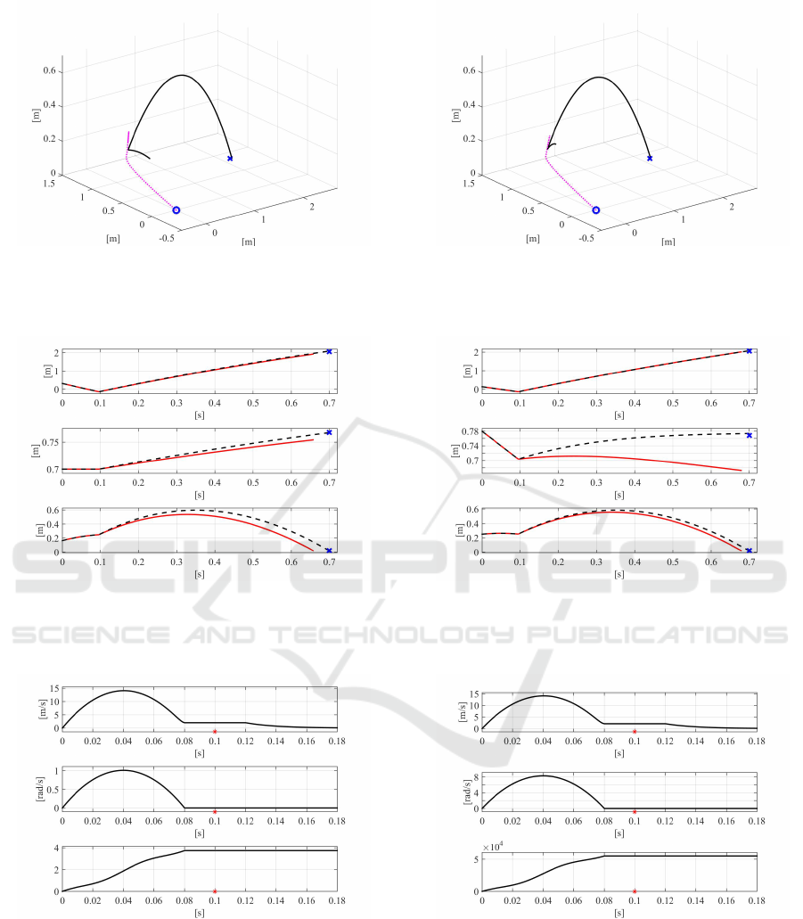
The results obtained for each of the three case

studies are depicted by their time histories in Fig-

ures 4, 5 and 6, respectively. In particular, the 3D

trajectories of both the ball and the paddle are rep-

resented in Figures 4(a), 5(a) and 6(a), respectively.

The solid line represents the ball, while the paddle

is depicted by a dashed line. The time histories of

each component p

, p

and p

related to the tra-

jectory of the ball are represented in Figures 4(b), 5(b)

An Optimal Trajectory Planner for a Robotic Batting Task: The Table Tennis Example

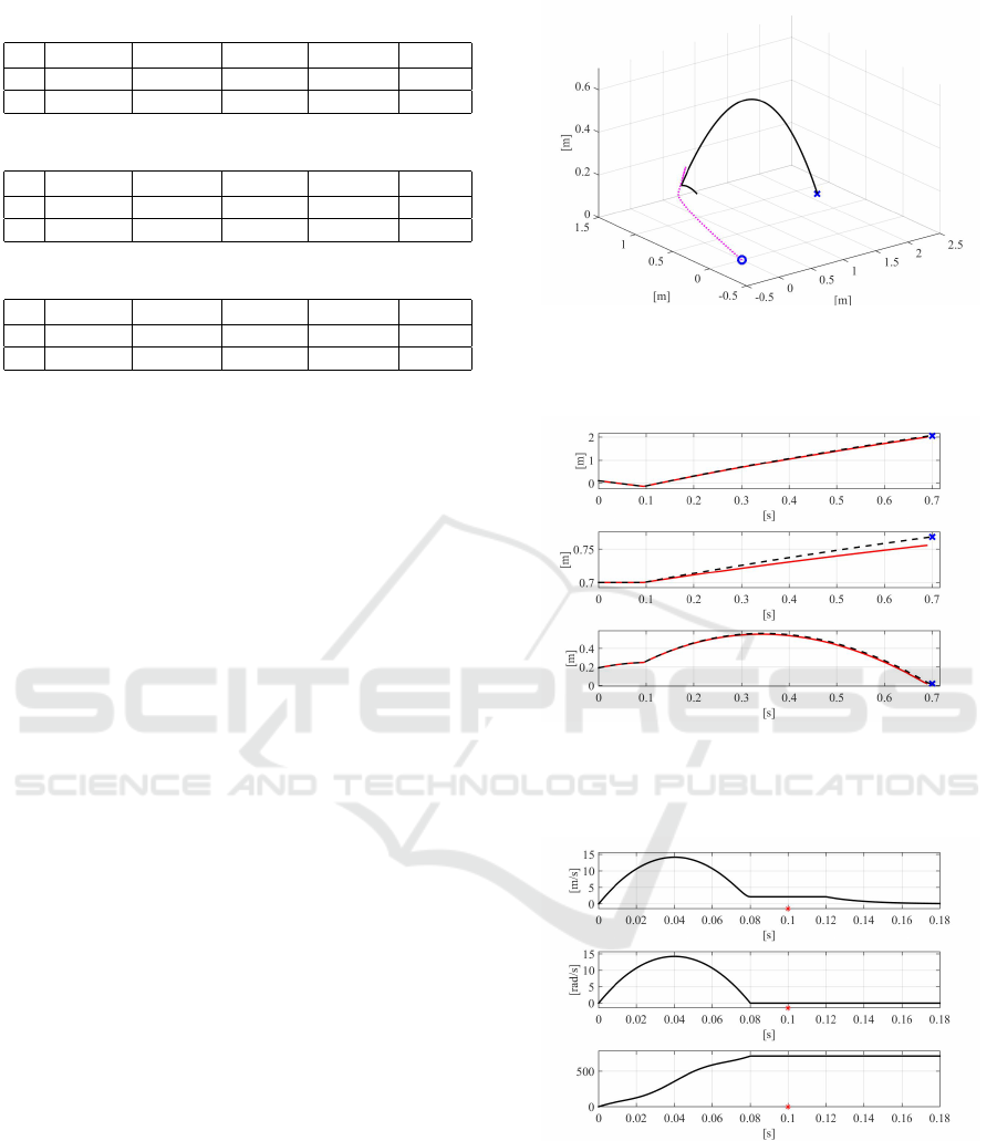
Table 3: Comparative case study 1 - Numerical results.

∆t

[s] ∆p

[m] ∆t

[s] ∆p

[m] t

[ms]

A 5.2e-3 1.3e-2 1.12e-2 5.47e-2 9e-3

B 5.14e-3 1.29e-2 4.88e-3 6.47e-4 21

Table 4: Comparative case study 2 - Numerical results.

∆t

[s] ∆p

[m] ∆t

[s] ∆p

[m] t

[ms]

A 3.86e-3 1.74e-2 4.26e-2 1.3e-1 8e-3

B 4.01e-3 1.81e-2 7.34e-4 3.29e-2 21

Table 5: Comparative case study 3 - Numerical results.

∆t

[s] ∆p

[m] ∆t

[s] ∆p

[m] t

[ms]

A 4.88e-3 1.42e-2 2.12e-2 1.03e-1 1e-2

B 4.86e-3 1.41e-2 9.02e-4 1.94e-2 25

and 6(b), respectively, for both of the compared meth-

ods: the solid line graphs the solution obtained by ex-

ploiting the method described by (Liu et al., 2012),

while the dashed curve illustrates the trajectory of the

ball obtained using the proposed method. The ﬁgures

indicate that the proposed method yields an improve-

ment over (Liu et al., 2012) by directing the ball closer

to the goal conﬁguration.

The quantitative results for the backspin, topspin

and sidespin case studies are shown in Tables 3, 4

and 5, where A represents the results obtained em-

ploying the Liu’s planner, whereas B the results ob-

tained employing our planner. The ﬁrst two columns

of each of the aforementioned tables refer to the preci-

sion of the impact. In both the approaches the results

are very similar. The gist of the comparison may be

captured by analyzing the last three columns of these

tables. The ﬁnal time error is reduced by about an

order of magnitude. The Euclidean norm of the er-

ror between the actual ﬁnal position of the ball and

the desired one is smaller by about an order of mag-

nitude, too.

Unfortunately, experiments are not yet available

for the proposed approach since the practical set-up

is under development. However, the switching from

Matlab into C++ language is already accomplished.

The computational time t

required to solve at run-

time both the simpliﬁed aerodynamic model and the

complete one is show in the last column of Tables 3,

4 and 5. The code is running on a computer with

speciﬁcations Intel Core 2 Quad CPU Q6600 @ 2.4

GHz, Ubuntu 12.04 32-bit operating system, includ-

ing the Levenberg-Marquardt C++ library (Lourakis,

2004). The same numerical results obtained with

Matlab have been retrieved, but the evaluation of the

computation burden is more precise, in the sense that

it is the one that will appear during the practical exper-

iments. To elaborate, compared to (Liu et al., 2012),

the prosented method increases the accuracy of the ﬁ-

(a) 3D trajectories of the ball, solid line, and the paddle,

dashed line, obtained with the proposed method. The

blue circle represents the initial position of the paddle,

while the blue cross is the desired ﬁnal position of the

ball.

(b) Comparison between ball trajectories: the solution

given by analytically solving (6) is depicted through a

solid line, the proposed one is instead represented with

a dashed line. The blue cross represents the desired ﬁnal

position of the ball.

planned linear and angular velocity of the paddle, evalu-

ation of the acceleration functional J in (12) between the

motion plan devised using the Euler angles and the op-

timal proposed one. The red star represents the impact

time t

Figure 4: Comparative case study 1.

nal desired position an order of magnitude for topspin

and sidespin cases and two orders of magnitude for

the backspin case. Furthermore, the C++ implemen-

ICINCO 2016 - 13th International Conference on Informatics in Control, Automation and Robotics

(a) 3D trajectories of the ball, solid line, and the paddle,

dashed line, obtained with the proposed method. The

blue circle represents the initial position of the paddle,

while the blue cross is the desired ﬁnal position of the

ball.

(b) Comparison between ball trajectories: the solution

given by analytically solving (6) is depicted through a

solid line, the proposed one is instead represented with

a dashed line. The blue cross represents the desired ﬁnal

position of the ball.

planned linear and angular velocity of the paddle, evalu-

ation of the acceleration functional J in (12) between the

motion plan devised using the Euler angles and the op-

timal proposed one. The red star represents the impact

time t

Figure 5: Comparative case study 2.

tation of the proposed nonlinear minimization prob-

lem, which considers the full aerodynamic model of

the ball, takes about 20 ms to give the desired veloc-

(a) 3D trajectories of the ball, solid line, and the paddle,

dashed line, obtained with the proposed method. The

blue circle represents the initial position of the paddle,

while the blue cross is the desired ﬁnal position of the

ball.

(b) Comparison between ball trajectories: the solution

given by analytically solving (6) is depicted through a

solid line, the proposed one is instead represented with

a dashed line. The blue cross represents the desired ﬁnal

position of the ball.

planned linear and angular velocity of the paddle, evalu-

ation of the acceleration functional J in (12) between the

motion plan devised using the Euler angles and the op-

timal proposed one. The red star represents the impact

time t

Figure 6: Comparative case study 3.

ity of the ball after the impact. This duration is grater

than what is shown in (Liu et al., 2012), but it is still

acceptable for real-time implementation.

An Optimal Trajectory Planner for a Robotic Batting Task: The Table Tennis Example

6.3 Optimal Planner Simulations

For each case study, the paddle trajectory is planned

over the time interval [t

] = [t

− ε], where ε =

0.02 s. The paddle trajectory is supposed to start still,

from the origin of the world frame, with initial ori-

entation R

= R

(π/2)R

(0), without loss of gener-

ality. According to the proposed algorithm, the posi-

tion, orientation and linear velocity of the paddle at

the impact time are given by the ball reset map solu-

tion. The Euclidean norm of the linear and angular

velocities of the paddle, planned with the minimum

total acceleration, are represented by the top and mid-

dle plots in Figures 4(c), 5(c), 6(c) and 3(b), for each

simulation.

Once the desired orientation is achieved with zero

angular velocity, the angular acceleration is set to

zero so that the orientation of the paddle remains the

same until the impact occurs. As long as one has

the control authority at the torque level, this con-

trol strategy, which switches only once, is straight-

forward to implement. Once the impact has occurred

at time t

, notice that the linear velocity of the pad-

dle is exponentially dissipated by the following term

exp(−µ(t −(t

+ δ))), where t is the time, µ = 50 and

δ = 0.02, so that the paddle stops.

The optimal trajectory discovered by solving the

two-point boundary value problem (14) indeed min-

imizes the L

norm of the total acceleration of the

paddle. So as to illustrate this fact, another typical

trajectory for the orientation of the paddle is planned.

This alternative plan constructs a third-order polyno-

mial function for the Euler angles, φ and θ, such that

the initial and ﬁnal orientation and angular velocity

constraints are satisﬁed. Both the angular acceler-

ation that corresponds to this motion plan and the

acceleration functional J in (12) are then computed.

For each case study, the bottom time histories of Fig-

ures 3(b), 4(c), 5(c) and 6(c), depict the value of the

difference of the acceleration functional between the

motion plan devised using the Euler angles and the

optimal motion plan. Notice that the value of this cost

functional is positive at t = t

, indicating that the opti-

mal motion plan indeed yields a smaller value of the

acceleration functional than a typical plan performed

using polynomials on the Euler angles, φ and θ.

About the computational burden of the proposed

planner, the code has been translated in C++ and eval-

uated on the same PC as in Section 6.2. The boundary

value problem for the optimal paddle trajectory plan-

ner takes less than 30ms. To sum up, after the high-

speed vision system gives a stable trajectory estima-

tion of the ball coming towards our court, it is possi-

ble to compute the desired trajectory for the paddle in

50ms (20ms + 30ms), hitting the ball with a proper ve-

locity to redirect it to the opposite court at the desired

position with the imposed spin. Another possibility

is that, once the desired impact position, velocity and

orientation is determined, one can immediately start

controlling the paddle to achieve these via a PD con-

troller, and revert to a trajectory following controller

once the optimal trajectory is available and is period-

ically updated.

7 CONCLUSIONS AND FUTURE

WORK

The presented paper proposes an algorithm to plan a

robotic batting task. In particular, a table tennis game

performed by a robot has been considered. The pro-

posed solution improves the control accuracy while

dealing with the real-time constraint. A coordinate-

free, smooth, optimal motion plan, that minimizes the

acceleration functional of the paddle, is proposed. As

future work, the proposed technique is planned to be

validated through experimental studies. Different op-

timal planners which make use of the dynamic model

of the robotic manipulator grasping the paddle may

also be considered.

ACKNOWLEDGEMENTS

The research leading to these results has been sup-

ported by the RoDyMan project, which has re-

ceived funding from the European Research Council

FP7 Ideas under Advanced Grant agreement number

320992.

REFERENCES

Acosta, L., Rodrigo, J., Mendez, J., Marichal, G. N., and

Sigut, M. (2003). Ping-pong player prototype. IEEE

Robotics & Automation Magazine, 10(4):44–52.

Andersson, R. (1989a). Aggressive trajectory generator for

a robot ping-pong player. IEEE Control Systems Mag-

azine, 9(2):15–21.

Andersson, R. (1989b). Dynamic sensing in a ping-pong

playing robot. IEEE Transactions on Robotics and

Automation, 5(6):728–739.

Cigliano, P., Lippiello, V., Ruggiero, F., and Siciliano, B.

(2015). Robotic ball catching with an eye-in-hand

single-camera system. IEEE Transactions on Control

Systems Technology, 23(5):1657–1671.

do Carmo, M. (1992). Riemannian Geometry. Mathematics

(Boston, Mass.). Birkh

auser.

ICINCO 2016 - 13th International Conference on Informatics in Control, Automation and Robotics

100

Huang, Y., Xu, D., Tan, M., and Su, H. (2013). Adding

active learning to LWR for ping-pong playing robot.

IEEE Transactions on Control Systems Technology,

21(4):1489–1494.

Kuka (2014). The Duel: Timo Boll vs. KUKA Robot. [web

page] https://youtu.be/tIIJME8-au8+.

Lippiello, V. and Ruggiero, F. (2012). 3D monocular

robotic ball catching with an iterative trajectory esti-

mation reﬁnement. In IEEE International Conference

on Robotics and Automation, pages 3950–3955, Saint

Paul, MN, USA.

Liu, C., Hayakawa, Y., and Nakashima, A. (2012). Racket

control and its experiments for robot playing table ten-

nis. In IEEE International Conference on Robotics

and Biomimetics, pages 241–246, Guangzhou, CN.

Lourakis, M. (Jul. 2004). levmar: Levenberg-Marquardt

nonlinear least squares algorithms in C/C++. [web

page] http://www.ics.forth.gr/ lourakis/levmar/+. [Ac-

cessed on 31 Jan. 2005.].

Lynch, K. and Mason, M. (1999). Dynamic nonprehen-

sile manipulation: Controllability, planning, and ex-

periments. The International Journal of Robotics Re-

search, 18(64):64–92.

Matsushima, M., Hashimoto, T., Takeuchi, M., and

Miyazaki, F. (2005). A learning approach to

robotic table tennis. IEEE Transactions on Robotics,

21(4):767–771.

uller, M., Lupashin, S., and D’Andrea, R. (2011).

Quadrocopter ball juggling. In IEEE/RSJ Interna-

tional Conference on Intelligent Robots and Systems,

pages 5113–5120, San Francisco, CA, USA.

ulling, K., Kober, J., Kroemer, O., and Peters, J. (2013).

Learning to select and generalize striking movements

in robot table tennis. The International Journal of

Robotics Research, 32(3):263–279.

ulling, K., Kober, J., and Peters, J. (2010). A biomimetic

approach to robot table tennis. In IEEE/RSJ Interna-

tional Conference on Intelligent Robots and Systems,

pages 1921–1926, Taipei, TW.

Nakashima, A., Ito, D., and Hayakawa, Y. (2014). An on-

line trajectory planning of struck ball with spin by ta-

ble tennis robot. In IEEE/ASME International Con-

ference on Advanced Intelligent Mechatronics, pages

865–870, Besanc¸on, F.

Nakashima, A., Ogawa, Y., Kobayashi, Y., and Hayakawa,

Y. (2010). Modeling of rebound phenomenon of

a rigid ball with friction and elastic effects. In

IEEE American Control Conference, pages 1410–

1415, Baltimore, MD, USA.

Nonomura, J., Nakashima, A., and Hayakawa, Y. (2010).

Analysis of effects of rebounds and aerodynamics for

trajectory of table tennis ball. In IEEE Society of

Instrument and Control Engineers Conference, pages

1567–1572, Taipei, TW.

Omron (2015). CEATEC 2015: Omron’s Ping Pong Robot.

[web page] https://youtu.be/6MRxwPHH0Fc+.

Oubbati, F., Richter, M., and Schoner, G. (2013). Au-

tonomous robot hitting task using dynamical sys-

tem approach. In IEEE International Conference on

Systems, Man, and Cybernetics, pages 4042–4047,

Manchester, UK.

Senoo, T., Namiki, A., and Ishikawa, M. (2006). Ball con-

trol in high-speed batting motion using hybrid trajec-

tory generator. In IEEE International Conference on

Robotics and Automation, pages 1762–1767, Orlando,

FL, USA.

Serra, D., Satici, A. C., Ruggiero, F., Lippiello, V., and Si-

ciliano, B. (2016). An optimal trajectory planner for a

robotic batting task: The table tennis example. [web

page] https://youtu.be/GXtBvbUHu5s+.

Silva, R., Melo, F., and Veloso, M. (2015). Towards ta-

ble tennis with a quadrotor autonomous learning robot

and onboard vision. In IEEE/RSJ International Con-

ference on Intelligent Robots and Systems, pages 649–

655, Hamburg, D.

Wei, D., Guo-Ying, G., Ye, D., Xiangyang, Z., and Han,

D. (2015). Ball juggling with an under-actuated ﬂying

robot. In IEEE/RSJ International Conference on In-

telligent Robots and Systems, pages 68–73, Hamburg,

Yanlong, H., Bernhard, S., and Jan, P. (2015). Learning

optimal striking points for a ping-pong playing robot.

In IEEE/RSJ International Conference on Intelligent

Robots and Systems, pages 4587–4592, Hamburg, D.

Zefran, M., Kumar, V., and Croke, C. (1998). On the gen-

eration of smooth three-dimensional rigid body mo-

tions. IEEE Transactions on Robotics and Automa-

tion, 14(4):576–589.

Zhang, Y., Xiong, R., Zhao, Y., and Chu, J. (2012). An

adaptive trajectory prediction method for ping-pong

robots. In Intelligent Robotics and Applications, pages

448–459. Springer.

An Optimal Trajectory Planner for a Robotic Batting Task: The Table Tennis Example

101