Evolutionary Optimization Algorithms for Differential Equation

Parameters, Initial Value and Order Identification

Ivan Ryzhikov, Eugene Semenkin and Ilia Panfilov

Institute of Computer Sciences and Telecommunication, Siberian State Aerospace University,

Krasnoyarskij Rabochij. 31, Krasnoyarsk, 660014, Russian Federation

Keywords: Dynamic System, Linear Differential Equation, Evolutionary Strategies, Parameters Identification, Initial

Value Estimation, Order Estimation.

Abstract: A dynamic system identification problem is considered. It is an inverse modelling problem, where one

needs to find the model in an analytical form and a dynamic system is represented with the observation data.

In this study the identification problem was reduced to an optimization problem, and in such a way every

solution of the extremum problem determines a linear differential equation and coordinates of the initial

value. The proposed approaches do not require any assumptions of the system order and the initial value

coordinates and estimates the model in the form of a linear differential equation. These variables are

estimated automatically and simultaneously with differential equation coefficients. Problem-oriented

evolution-based optimization techniques were designed and applied. Techniques are based on the

evolutionary strategies algorithm and have been improved to achieve efficient solving of the reduced

problem for every proposed determination scheme. Experimental results confirm the reliability of the given

approach and the usefulness of the reduced problem solving tool.

1 INTRODUCTION

The dynamical system identification problem is not

new but is still of current importance; it is being

investigated and developed. There are many

different problem definitions and many applications

for the problem. Chemistry, biology, engineering

and econometrics are the scientific fields in which

dynamic system modelling is useful. Some problems

are related to linear differential equations.

This study is focused on the identification

problem, in the case of making the model with only

the output observations of the object and a control

function known. A linear differential equation is

used as a mathematical model of the dynamic

process. It is important to point out that generally

there is no information about the order of the

equation and its initial value coordinates. The

observations are the distorted measurements of the

system output. Many other approaches to the

identification receive the model in the form of an

adequate approximation of the system trajectory. But

for some objects it is necessary to have a model that

determines dynamic system behaviour. For this

reason the solution of the identification problem is

required to be in a symbolic form. It permits the

model to be useful in further research or work. The

model in the form of the differential equation gives

the opportunity to solve the optimal control problem,

predict system behaviour and conduct stability

analysis among other things.

There are many studies on identification

problems and the estimation of the differential

equation parameters. So-called inverse problems

occur for different models: linear differential

equations, partial differential equations, nonlinear

and delay differential equations.

Our work is related to the identification of single

input and single output systems. The proposed

approach is also a useful tool for making a

linearization of any dynamic process, despite its

nature.

The problem of parameter and initial value

estimation in the case of a known structure is also a

complex problem and many approaches are being

developed. Some approaches are based on the pre-

processing of sample data (Fang et al., 2011), (Wu et

al., 2012). Also there is a class of approaches which

are based on the shooting or multiple shooting idea,

(Peifer et al., 2007), or nonparametric estimation

168

Ryzhikov, I., Semenkin, E. and Panﬁlov, I.

Evolutionary Optimization Algorithms for Differential Equation Parameters, Initial Value and Order Identiﬁcation.

DOI: 10.5220/0005979201680176

In Proceedings of the 13th International Conference on Informatics in Control, Automation and Robotics (ICINCO 2016) - Volume 1, pages 168-176

ISBN: 978-989-758-198-4

(Brunel, 2008). In the paper (Schenkendorf et al.,

2014) flatness was used for parameter identification

problem solving for ordinary differential equations

(ODE) and ODE with a delay. There are many

works on parameter estimation in the case when the

equation structure is given, i.e. (Wöbbekind et al.,

2013). All that is mentioned here proves the

importance of the dynamic system identification

problem. A genetic algorithm is applied to the

parameters identification problem for ODE (Sersic

et al., 1999), but the structure of the system is given.

A genetic algorithm was also used in the study

(Parmar et al., 2007), in which an order reduction

problem is considered and the model is a second

order linear differential equation. But the

discretization of real values results in a significant

limitation in applicability, and algorithms of this

nature do not satisfy the needs of the considered

identification problem. Another powerful nature-

inspired optimization algorithm, partial swarm

optimization, was applied to nonlinear dynamical

system linearization, (Naiborhu et al., 2013).

Our approach is based on the reduction of the

identification problem to the extremum problem on

the real-value vector space or on the space with real

and integer vector coordinates. The problem

reduction allows the simultaneous estimation of the

coefficients, the initial value and the order of the

differential equation. The objective functional

requires a powerful optimization tool. The results of

previous work allow us to conclude that improved

evolution-based optimization techniques are

workable and reliable tools and can be applied to

this class of optimization problem.

Optimization algorithms were improved; search

operators were designed and implemented. Criteria

for comparing algorithms and estimating efficiencies

were proposed. The performance of algorithms was

investigated and examined on a set of identification

problems.

2 IDENTIFIACTION PROBLEM:

ORDER, COEFFICIENTS,

INITIAL POINT

Let a set





,, , 1,

iii

yut i s , be a sample, where

yR

is the dynamic system output measurement

at the time point

()

uut

is a control action and

is the size of the sample. In the current

investigation it is supposed that the control function

()ut

is known. It is also proposed that the object to

be identified can be described with a linear

differential equation of unknown order, and its

system state is a solution of the Cauchy problem:

() ( 1)

()

ax a x axbut



 

(0)



(1)

As can be seen, solving the identification problem

requires the initial value

if it is necessary to find

a solution in a symbolic form, in the form of a linear

differential equation (LDE). In the case of distorted

observations and/or a small sample size it is a

difficult problem to estimate the coordinates of the

initial value vector and some approaches can result

in significant errors in estimated derivative values.

Thus it is important to develop an approach to

estimate simultaneous initial value coordinates and

the LDE coefficients and order.

It is assumed, that the output data

___

,1,

yi s

distorted by additive noise

:() 0, ()ED



 

___

() , 1,

iii

yxt i s

(2)

where the

()

function is a solution of the Cauchy

problem (1).

Without loss of generality, one may assume that

the system is described with the following

differential equation:

() ( 1)

()

kkk

xxut

aaa



 

(3)

() ( 1)

()

ax axaut



 



 .

(4)

Let m be the order of the LDE, which is assumed to

be limited,

,mM



and ,

MN is the parameter

that one can set to limit the maximum order. We

seek the solution of the identification problem as the

LDE, and it is determined with the following

parameters: order

,mM

coefficients



ˆˆ ˆˆ

,,,

aa aa R





and initial value

vector

(0)

R . It is proposed to estimate the

adequacy of a model by comparing the sample data

with the solution of the Cauchy problem:

() ( 1)

ˆˆˆ ˆˆˆ

()

ax axaut



  ,

(0)



(5)

The current problem is the extension of earlier work,

which is focused on LDE order and coefficient

estimation, (Ryzhikov et al., 2013). Our approach

Evolutionary Optimization Algorithms for Differential Equation Parameters, Initial Value and Order Identiﬁcation

169

meets three ways of LDE determination. The first is

based on the following representation of a solution.

Let a vector



ˆˆˆˆ

0...0 , , ,

aaaaR





be a

form of determination for both variables m and

For the order

m vector

will contain



zero

coordinates from the origin. Now when

m is

defined by the variable

, let

R be a vector

of initial value coordinates and

R - its first m

coordinates. Now the identification problem solution

is determined by the values that deliver an extremum

to a functional

ˆˆ ˆ

,(0)

(, ) () min

aax x

aR x R

Iax y xt









 



(6)

where

ˆˆ

,(0)

()

aax x



is a solution of the Cauchy

problem (5) with order

m , coefficients

determined by

aa

and initial point

ˆˆ

(0)



determined by

Thus, the simultaneous estimation of all the

parameters leads to extremum problem solving on





Another method of determination is based on the

assumption that coefficient

b of control function (3)

is not equal to 0. Thus, the same differential

equation can be represented in a different way

() ( 1)

ˆˆ ˆ

()

aa a

xxut

bb b



  

(7)

() ( 1)

ˆˆ ˆ

()

ax a x axut



 

 

 .

This representation leads to the same optimization

problem (6).

Both solution representations have their

disadvantages, which are related to the impossibility

of transforming the vector into some class of

equations. For the determination based on equation

(4) it is impossible to determine a differential

equation of order



with





. For the other

method of determination it is impossible to

determine a differential equation with a control

coefficient that is equal to 0.

One more method of determination is based on

the representation of LDE with a vector





and an integer

mM . The integer variable value

sets the order and determines the number of

elements for both vectors



 and

R .

The criterion for this method of determination is

suggested to be the following:

ˆˆˆ

(, 1),(0) ( , )

(, , ) ()

afam x fx m

Iax m y xt









(, , ) min

aR x R mM

Iax m







(8)

where

dim( ) dim( )

(,): , (,)

zzi

fxn R R fxn













is a function, that transforms the vectors so its

coordinates that do not fit the order are equal to 0.

The current determination leads to the optimization

problem in





RRxNxM



 

3 MODIFIED HYBRID

EVOLUTIONARY STRATEGY

ALGORITHM FOR LDE

IDENTIFICATION

Evolution-based extremum seeking techniques are a

useful tool for solving multimodal and complex

black-box optimization problems. This is the reason

the evolution strategy approach was suggested as the

basic one. The evolution strategy optimization

algorithm is widely applied and its efficiency has

been proved. Its principles are described in

(Schwefel, 1995).

Some classes of optimization problems have

specific features, so it is possible to analyse

properties and reveal the way of improving the

techniques that one can use to solve these problems.

Since the proposed functional (6) is complex,

because of the way the LDE order is determined and

parameters and initial values are determined with

one vector, some necessary implementations and

modifications were made to improve the approach

performance. Every alternative is an individual and

is characterized by the value of its fitness. The

fitness function of individual

X is a mapping

()

1( arg())





(9)

arg( )

I is a transformation of the individual’s

vector coordinates to the arguments of the functional

(6) or (8).

In the current investigation the evolutionary

strategy optimization algorithm was implemented

with the following features: 3 selection schemes:

tournament, proportional and rank; 6 crossover

schemes; 2 mutation schemes.

The crossover operator is determined by one of

the expressions:

ICINCO 2016 - 13th International Conference on Informatics in Control, Automation and Robotics

170









(10)







_____

,1,

cs p

Pi i j n



 



(11)

where

is an offspring,

i is one of the parents,

n is the a quantity of parents, w is the weight

coefficients.

Crossover schemes differ in their way of forming

offspring: as a weighted average of its parents (10)

or when every offspring’s gene has the probability to

be equal to one of the parents’ genes.

Here we describe some standard and suggested

methods of weight determination. For the case (10):

 ,





wfi

(min ,1)

wU

(min , ( ))

jcs

wU fi

; and for the case (11):

 ,

(min , ( ))

jcs

wU fi

. In the given

expressions

(,)Uab is a uniform distribution on





,ab

min

is a crossover parameter that prevents

dividing by 0.

The first essential improvement is the

implementation of a stochastic extremum seeking

algorithm as a searching operator that acts after

standard operators in every generation. The designed

stochastic local optimization algorithm is similar to

the coordinate-wise extremum seeking technique.

The aim of its implementation is to improve

alternatives after the random search. The suggested

local optimization algorithm is controlled by 4

parameters:

N - the number of individuals to be

optimized,

N - the number of genes to be

improved,

- the number of steps for every gene,

and

- optimization step value.

The second modification is related to the

suppressing of the mutation influence. It is an

important point, because the way of transforming the

objective vector into a differential equation makes

the problem very sensitive to even small changes of

the alternative variables. Thus, it was suggested, to

add the probability for every gene to be mutated, so

that one can decrease the mutation by lessening the

value of this setting

. Let the optimization

problem dimension be

dim( )Nx

, variable





...

rr r

is randomly distributed for every

individual and









01 , 1

mj m

Pr p Pr p 

Now the mutation operator can be described as

follows, for counter

____

1,jN

   





0, ,

mcj c

jj jN

iirNi





(12)







 







0,1

mjcjc

jN jN jN

iririe





   

(13)

 



0,1 ,

mcj

jN jN

iirN





(14)

where



____

,1,

ijN are objective parameters,



____

,1,

ijN



 are strategic parameters,



is a

learning coefficient,





,NE

is a normally

distributed random value with an expected value

and a variance



Another improvement also focused on supressing

the random search influence on the order estimation.

The vector determines LDE order and some of its

coordinates equal zeroes if

mM . However

efficient stochastic optimization algorithms for real

variables are based on adding some random values

to them. This leads to a contradiction. To solve it, a

rounding operator was suggested. One more

parameter sets the threshold level

t

, so the

rounding operator works as follows



 

_____

,1,

mml

m с

iifi t

ijN

otherwise















(15)

where

the number of objective parameters that

transform into ODE coefficients.

For the functional (8) and related transformation,

the modified algorithm was extended to solving

optimization problems with both real and integer

variables. To save the concept of the evolution

strategy algorithm, the integer variable is also

related to its strategic parameter.

Since the single input and single output

identification problem is considered, every

alternative consists of





real value variables

and one integer. The schemes of the crossover

operator are similar to (11).

Let

be the probability for one integer gene to

mutate. Let

123

mmm

rrr be a random variables:

Evolutionary Optimization Algorithms for Differential Equation Parameters, Initial Value and Order Identiﬁcation

171





01 ,

Pr p





Pr p













01min1,

Pr i













1min1,

Pr i

and



____

,1,

Pr j j N

  . The mutation operator

works similarly to (12) and (13):









123 12

(1 )

mmmm mmm

irrr rri  ,

(16)









(0,1)

mmmc

iirN

(17)

The main benefit of implementing all the

modifications is to achieve a sufficient improvement

of the algorithm efficiency. For the same

computational resources all of these algorithms are

more reliable and more efficient than the standard

differential evolution algorithm, particle swarm

optimization algorithm and evolutionary strategies

with covariance matrix adaptation. The

modifications were designed to lessen the

complexity that arises from the vector-to-model

transformation and the requirements of simultaneous

parameter estimation.

4 PERFORMANCE

INVESTIGATION

To make an investigation of the algorithms and

estimate their performances we need to put forward

criteria. The first criterion is basic and related to the

value (6) for models in forms (7) and (5) and with

value (8) for the approach that includes integers and

real values. To simplify the representation of results,

let

be the criterion (6) or (8), depending on what

algorithm was used.

Another criterion calculates the distance between

the model output and the real output; we denote it

. It is also important to calculate the error in LDE

parameter estimation

, in the case of the real

order being estimated.

() ()

Cxtxtdt



(18)

300

ˆˆ

С aa x x 

(19)

Since criterion (19) is useful only for some class of

solutions, let us put forward one more criterion that

estimates the probability to find the real order



(20)

where

is the number of solutions with the same

order as the real object and

is the number of

algorithm runs.

The dynamic system output is the Cauchy

problem solution on





0, T

for the LDE with given

coefficients and the initial value. The solution needs

to be discretised and represented as a set with

elements. Let

be a set of randomly chosen

different integers, so accordingly to (2),



yx N













and





, where a

counter

1,is .

The list of differential equations that was used to

simulate the dynamic process is given in table 1. On

the basis of the given differential equations we form

initial problems and generate the observations. The

samples count 100 observations. The list of

problems is given in Table 1.

One faces a difficulty in the examination of

algorithms, caused by a large number of setting

combinations and a wide problem field. The latter

means that optimization problems have many

characteristics themselves and depend on differential

equations that determine the system output, sample

size, noise level and the way random numbers are

generated. Every setting and even every realisation

is a different problem, because the generating of a

sample is a random event.

Due to results of previous works it was decided

to use the following settings in the current

investigation: 100 individuals for 100 populations,

tournament selection, 3 parents for random

crossover, mutation scheme (12) and (14), the

mutation probability

 ,

N  individuals

for the local stochastic improvement,



genes and

1, 0.1

Nh, the threshold for

rounding

0.4



. For integer variables the mutation

setting took

 .

The strategic parameter of the initial population

were uniformly generated,





0,1U

, every objective

parameter is equal to 0, the integer variable with

equal probability takes a value from 1 to

. The

order limitation value took 10. Every algorithm was

launched 25 times for every identification problem.

ICINCO 2016 - 13th International Conference on Informatics in Control, Automation and Robotics

172

The algorithm that is based on the model (5) is

denoted as 1, the algorithm that is based on the

model (7) is denoted as 2 and the algorithm that

estimates the order with an integer variable is

denoted as 3. At first we examine algorithms on the

set of problems in Table 1. Results of the

examination are given in Table 2.

Table 1: Identification problems.

Identification problems

2()

xxut

 

  



2 0 , 12.5

xT

2()

xxut

 

  



2 2 , 12.5

xT 

2()

xxxut

  





0 1 0 , 12.5

xT

2()

xxxut

  





311 , 12.5

xT

2()

xxxut

  





2 0 0 , 12.5

xT

2()

xxut

 

  



01 , 12.5

xT

37 ()

xxut

 

 



3 3 , 12.5

xT 

23 ()

xxxut

  

   



111 , 12.5

xT  

(4)

2.2 3.5 ( )

xxxxut

  

  



2000 , 12.5

xT

(4)

2452()

xxxxut

  

    ,



0000 , 12.5

xT

(4)

43 ()

xxxxut

  

 ,



1000 , 12.5

xT

(4)

43 ()

xxxxut

  

 ,



2 0 0 0 , 12.5

xT

(5) (4)

0.6 3.4 1.1 2.4

xxxx



  

 

0.4 ( )

ut



00000 , 25

xT

(5) (4)

423

xxxx

  



0.5 ( )

ut



00000 , 25

xT

(6) (5) (4)

1.5 2 2 0.5

xxxx x

  

  

0.1 ( )

ut



000000 , 25

xT

Average values of criteria show that for the given

problems and samples, algorithm 1 is the most

efficient.

Table 2: Experimental results for different algorithms and

problems from the list in Table 1.

Algorithm

number

Criteria average values

1 0,045 0,996 0,399 0,441

2 0,059 1,287 3,349 0,453

3 0,057 1,180 0,389 0,252

Algorithm

number

Criteria value variance

1 0,017 0,335 1,246

2 0,007 1,520 3,040

3 0,003 0,566 0,508

Since observations of the system trajectory are

distorted, two more criteria were added. One is

needed to estimate the probability of finding a model

that is better than the system trajectory in fitting the

sample data



(21)

where

is the number of launches in which such

solutions were received. And the last criterion gives

us a difference in

criterion values for the model

and the object:

61 1

model object

С CC

(22)

where

model object

CC

and

model object

are the

criterion values for the model output and the system

output, respectively.

The next examination is related to an estimation

of noise level influence on the performance of the

algorithms. Results for problems 1, 5 and 12 from

Table 1 for different noise levels are demonstrated in

Table 3.

Table 3: Experimental results for different noise levels.

Averaged criteria values. Problems 1, 5 and 12, Table 1.

Alg.

Criteria average values

1 0,195 0,864 0,342 0,364 0,666 0,301

2 0,182 1,018 0,888 0,453 0,866 0,038

3 0,187 1,112 0,308 0,466 0,649 0,014

Alg.

Criteria variance

1 0,139 0,343 0,818 0,0004

2 0,008 0,251 2,118 0,006

3 0,007 0,209 0,468 0,004

As one can see algorithm 3 is the best for

criterion

values. But Table 3 shows that

algorithm 1 is still the most reliable: it has the

Evolutionary Optimization Algorithms for Differential Equation Parameters, Initial Value and Order Identiﬁcation

173

biggest average value of criterion

. The estimation

of its probability to find a solution that would fit the

observations more than the real system state equals

1. This can be interpreted as this algorithm finding a

solution that fits the sample data even better than the

real system output trajectory.

The value that the criterion (18) takes is also

important and is given in Figure 1 – its average

value for problems 1, 5 and 12. In these pictures, the

horizontal axis is the noise level and the vertical axis

is the average value of the criterion (18) for 25

launches.

Figure 1: Problems 1, 5 and 12, criterion (18) average

value for different noise levels.

The next examination aim is to investigate the

effect of the sample size on the algorithm

performance. The sample size was varied from 90 to

5: 90, 80, …, 20, 15, 10, 5. All the average criteria

values are given in Table 4 for problems 1, 5 and 12

and 25 launches of the algorithms.

Table 4: Experimental results for different sample size

values. Problems 1, 5 and 12, table 1.

Algorithm

number

Criteria average values

1 0,013 0,398 0,596 0,288

2 0,013 0,464 0,502 0,613

3 0,021 0,549 0,286 0,482

Algorithm

number

Criteria variance

1 0,009 0,210 0,408

2 0,014 0,530 0,995

3 0,010 0,440 0,464

A criterion (18) average value for different

sample size is presented in Figure 2.

Figure 2: Problems 1, 5 and 12, criterion (18) average

value for different sample size.

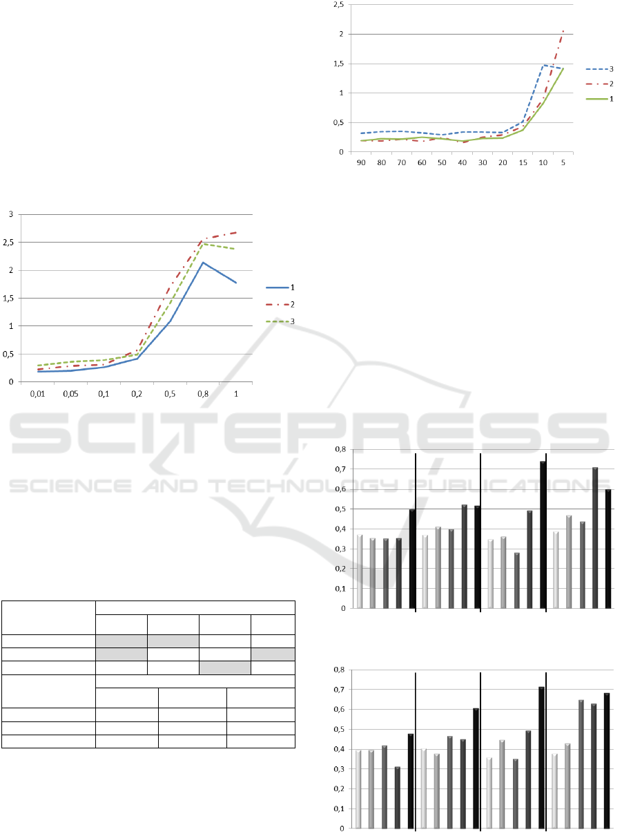
To estimate the influence of both factors: sample

size and noise level, another examination was

performed. The noise level took values 0.01, 0.05,

0.1, 0.2, 0.3 and the sample size was varied: 200,

150, 80, 40. There we consider all three algorithms

for problems 1, 5 and 12. Figures 3, 4 and 5

represent the average values of criterion

for the

algorithm 1, 2 and 3, respectively. To make a better

presentation of the results, statistics for every sample

size are given in a distinct area in the figures. The

bars represent average values for some sample size

and noise level, differ in colour; the darker colour

matches the higher noise level.

Figure 3: Criterion (18) average value for different noise

levels and sample sizes. Algorithm 1.

Figure 4: Criterion (18) average value for different noise

levels and sample sizes. Algorithm 2.

200 150 80 40

ICINCO 2016 - 13th International Conference on Informatics in Control, Automation and Robotics

174

Figure 5: Criterion (18) average value for different noise

levels and sample sizes. Algorithm 3.

Increasing the noise level and decreasing the

sample size leads to a loss in efficiency. However

the estimation of probabilities

and

shows us

the algorithms find a good solution. The samples are

not representative, so it is impossible to identify the

real dynamical system. Only the dynamical system

whose trajectory fits the data can be identified.

In this study the criterion (18) was suggested as

being the most important, because it is the

estimation of the output distance of the model from

the real system output. It is used since it is more

useful than criterion

for samples with noised

data. Yet it is impossible to use this criterion in

solving inverse mathematical modelling problems.

We also suggest that the criterion

could be used

instead of

, but it is more difficult to interpret the

results.

5 CONCLUSIONS

The approaches and algorithms described in this

work are proven to be useful for linear dynamic

system identification. The improved optimization

algorithms are powerful and reliable tools for

solving the reduced extremum problem. The

approach allows the inverse mathematical modelling

problem to be solved in a symbolic form knowing

only the control function. Since the approach and

algorithms solve the problem automatically and

simultaneously for all variables, the approach is

flexible. The designed algorithms can be easily

modified to seek solutions in cases where there is no

control input or where the initial value is given.

The developing of the dynamic system

identification problem solving approach requires

some specific criteria for estimating the optimization

algorithms. They are related to the complexity of the

problem and its features. In the current study we

suggested 6 criteria. Criteria allow algorithm

performance to be investigated and more

information about the features of a reduced problem

to be given. The data we received from the

experiments is useful for the further development of

evolutionary algorithms and dynamic identification

problem solving approaches.

New features of the reduced problem were

explored. In the case of no data distortion, the

sample size does not affect the efficiency. The

examination results show that the improved

optimization algorithms find a solution that fits the

sample better than the system output trajectory.

ACKNOWLEDGEMENTS

Research is performed with the financial support of

the Russian Foundation of Basic Research, the

Russian Federation, contract №20 16-01-00767,

dated 03.02.2016.

REFERENCES

Brunel N. J-B., 2008. Parameter estimation of ODE’s via

nonparametric estimators. Electronic Journal of

Statistics. Vol. 2, pp. 1242–1267.

Fang Y., Wu H., Zhu L-X., 2011. A Two-Stage Estimation

Method for Random Coefficient Differential Equation

Models with Application to Longitudinal HIV

Dynamic Data. Statistica Sinica. pp. 1145-1170.

Naiborhu J., Firman, Mu’tamar K., 2013. Particle Swarm

Optimization in the Exact Linearization Technic for

Output Tracking of Non-Minimum Phase Nonlinear

Systems. Applied Mathematical Sciences, Vol. 7, no.

109, pp. 5427-5442.

Parmar G., Prasad R., Mukherjee S., 2007. Order

reduction of linear dynamic systems using stability

equation method and GA. International Journal of

computer and Infornation Engeneering 1:1., pp.26-32.

Peifer M., Timmer J., 2007 Parameter estimation in

ordinary differential equations for biochemical

processes using the method of multiple shooting. IET

Syst Biol, pp. 78–88.

Ryzhikov I., Semenkin E., 2013. Evolutionary Strategies

Algorithm Based Approaches for the Linear Dynamic

System Identification. Adaptive and Natural

Computing Algorithms. Lecture Notes in Computer

Science, Volume 7824. – Springer-Verlag, Berlin,

Heidelberg, pp. 477-483.

Schenkendorf R., Mangold M., 2014. Parameter

identification for ordinary and delay differential

equations by using flat inputs. Theoretical

Foundations of Chemical Engineering. Vol. 48, Issue

5, pp. 594-607.

200 150 80 40

Evolutionary Optimization Algorithms for Differential Equation Parameters, Initial Value and Order Identiﬁcation

175

Schwefel Hans-Paul, 1995. Evolution and Optimum

Seeking. New York: Wiley & Sons.

Sersic K., Urbiha I., 1999. Parameter Identification

Problem Solving Using Genetic Algorithm.

Proceedings of the 1. Conference on Applied

Mathematics and Computation, pp. 253–261.

Wöbbekind M., Kemper A., Büskens C., Schollmeyer M.,

2013. Nonlinear Parameter Identification for Ordinary

Differential Equations. Proc. Appl. Math. Mech., 13:

pp. 457–458.

Wu H., Xue H., Kumar A., 2012. Numerical

Discretization-Based Estimation Methods for Ordinary

Differential Equation Models via Penalized Spline

Smoothing with Applications in Biomedical Research.

Biometrics, pp. 344-352.

ICINCO 2016 - 13th International Conference on Informatics in Control, Automation and Robotics

176