An Image Generator Platform to Improve Cell Tracking Algorithms

Simulation of Objects of Various Morphologies, Kinetics and Clustering

Pedro Canelas

, Leonardo Martins

, André Mora

, Andre S. Ribeiro

and José Fonseca

Computational Intelligence Group of CTS/UNINOVA, Faculdade de Ciências e Tecnologia,

Universidade Nova de Lisboa, Quinta da Torre, 2829-516, Caparica, Portugal

Laboratory of Biosystem Dynamics, Dep. of Signal Processing, Tampere University of Technology, Tampere, Finland

Keywords: Microscopy, Synthetic Time-lapse Image Simulation, Cell Tracking, Cluster Tracking.

Abstract: Several major advances in Cell and Molecular Biology have been made possible by recent advances in live-

cell microscopy imaging. To support these efforts, automated image analysis methods such as cell

segmentation and tracking during a time-series analysis are needed. To this aim, one important step is the

validation of such image processing methods. Ideally, the “ground truth” should be known, which is

possible only by manually labelling images or in artificially produced images. To simulate artificial images,

we have developed a platform for simulating biologically inspired objects, which generates bodies with

various morphologies and kinetics and, that can aggregate to form clusters. Using this platform, we tested

and compared four tracking algorithms: Simple Nearest-Neighbour (NN), NN with Morphology and two

DBSCAN-based methods. We show that Simple NN works well for small object velocities, while the others

perform better on higher velocities and when clustering occurs. Our new platform for generating new

benchmark images to test image analysis algorithms is openly available at

(http://griduni.uninova.pt/Clustergen/ClusterGen_v1.0.zip).

1 INTRODUCTION

Recent advances in live-cell microscopy imaging

have enabled the acquisition of images with higher

quality and resolution and the development of

techniques for detecting and observing recently

discovered cellular structures and their kinetics

(Danuser, 2011; Sung and McNally, 2011).

The main challenges in live-cell imaging can be

divided into two areas. The first relates to processes

that occur before and during image acquisition in the

microscope, associated with the refinement of

processes, such as illumination, focus, drift

correction, stage positioning and refinement of

microscope components (e.g. shutter, lens, camera,

stage) (Coutu and Schroeder, 2013). The second is

related to post processing limitations, associated

with storage of large amounts of data and image

processing (e.g., image registration, segmentation,

tracking, statistical quantification and background

correction) (Coutu and Schroeder, 2013; Bonnet,

2004).

Automatic correction algorithms are normally

included in microscope software packages (Frigault

et al., 2009), while the process of image registration

(overlaying two or more images of the same location

taken at different time frames and/or from different

viewpoints and/or by different sensorial devices) has

been extensively studied and several methods are

available. These are classified based on modality,

intensity, type of data, dimensionality, domain and

type of transformation, and registration

methodologies (Deshmukh and Bhosle, 2011;

Wyawahare et al., 2009).

The next step is related to the segmentation of

cells or cellular structures of interest (Meijering

2012), where these segmented objects are detected,

located, and separated from the background. The

main challenge is to automatize this process and

provide it with a high specificity and sensitivity for a

vast number of cases. Presently, most algorithms are

made available in open-source platforms and apply

several approaches, such as intensity thresholding,

feature detection, morphological filtering, region

accumulation, deformable model fitting, etc.

(Meijering, 2012).

When handling a time series, one needs to link

the segmented objects in the actual frame with the

ones from the previous frame, so as to extract the

Canelas, P., Martins, L., Mora, A., Ribeiro, A. and Fonseca, J.

An Image Generator Platform to Improve Cell Tracking Algorithms - Simulation of Objects of Various Morphologies, Kinetics and Clustering.

DOI: 10.5220/0005957800440055

In Proceedings of the 6th International Conference on Simulation and Modeling Methodologies, Technologies and Applications (SIMULTECH 2016), pages 44-55

ISBN: 978-989-758-199-1

object’s trajectory over time. Having available the

information describing the target, defined by the

state sequence X

, kϵ



(where



is the set of

frames), and the measurements defined by Z

, the

objective of tracking is to estimate X

, given all

measurements until the moment Z

1:k

(Tissainayagam

and Suter, 2005). This is made difficult by noise,

occlusions, illumination changes, complex motions

and object’s shape dynamics, which can enhance the

misidentification of object tracks over time (Yilmaz

et al., 2006).

Presently available tools for segmentation and

tracking in different microscopy settings include the

‘Cell-C’, based on DAPI staining and fluorescence

in situ hybridization images (Selinummi et al.,

2005), ‘CellTracer’, which applies morphological

methods to automatically segment bacterial cells,

yeast and human cells (Wang et al., 2010),

‘MicrobeTracker’ and its accessory tool

‘SpotFinder’, which segment Escherichia coli and

Caulobacter crescentus cells and detected

fluorescent spots within (Sliusarenko and Heinritz,

2011), ‘Schnitzcells’, which segments and tracks E.

coli cells in confocal or phase contrast images

(Young et al., 2012) and, ‘CellAging’, which was

developed for cell segmentation and tracking in

order to study the segregation and partitioning in cell

division of protein aggregates (Häkkinen et al.,

2013).

Validation of these image processing tools and

techniques they use require the use of gold-standard

images, usually manually annotated by biology

experts. This is problematic, as it is expert-

dependent (both inter-user and intra-user variability

can be high) and are impractical in high-throughput

data-sets (Coelho et al., 2009). To overcome this

problem, a viable alternative is to generate artificial

images using biologically inspired models. These

images, whose ground truth is known, can be used

for the accurate quantitative evaluation of image

processing algorithms (Bonnet, 2004).

In Section 2, we give a comprehensive literature

review of existing tools for simulation of synthetic

microscopy images and the recent developments on

cell tracking algorithms. In Section 3 we present the

contributions to the development of the image

simulation tool (models and parameters) and the

implementation of three different tracking

algorithms. In Section 4 the tracking results of

several examples are presented using different

parameters. Finally, in Section 5 we present final

remarks on the development of the simulation tool

and the results of the three algorithms, along

potential future endeavours.

2 STATE OF THE ART

2.1 Synthetic Image Generators

There have been several contests and open

challenges, usually requiring that each methodology

is tested on the same benchmark data-sets (acquired

by an independent laboratory or created by artificial

image generators) (Meijering, 2012). Such artificial

image generators require realistic biological models,

and commonly use theoretical and experimental

information regarding the statistical distributions of

the object’s behaviour (Xiong et al., 2010) but also

spatial and temporal data from the object (Kruse,

2012; Misteli, 2007). If the object studied is a cell,

these models should include morphology parameters

such as cell shape and size, location of subcellular

structures, kinetic and spatial statistics of cell

growth, cell division, cell migration and models of

internal cell functions.

The modus operandi of presently available tools

to simulate microscopy images based on biological

models can be divided in three stages: the digital

phantom object generation, the simulation of the

signal passing through the optical system and, the

simulation of the image formed on a specific sensor

(Svoboda et al., 2009).

Simulators such as ‘SIMCEP’ (Lehmussola et

al., 2007) have provided a gold-standard platform to

validate and test various image processing tools,

such as the previously mentioned ‘CellC’

(Selinummi et al., 2005), the open-source and Java-

based image processor ImageJ, and the

commercially available MCID Analysis (Imaging

Research Inc., Catharines, ON, Canada; Evaluation

ver. 7.0), along with other image processing tools

(Ruusuvuori et al., 2008). The phantom objects are

generated with different cell parameters, such as

probability of clustering, cell radius, and cell shape

and with parameters related to the sensors and the

optical system such as background noise and

illumination disturbance (Ruusuvuori et al., 2008;

Lehmussola et al., 2011).

Another toolbox, ‘CytoPacq’, was developed

specifically to simulate all three phases, by being

equipped with three different modules. The first

module (‘3D-cytogen’) generates the digital object

phantom, which imitates the cell structure and

behaviour and can generate microspheres,

granulocytes, HL-60 Nucleus and images of Colon

Tissue. The second module (‘3D-optigen’) simulates

the transmission of the signal through the lenses,

objective, excitation filter and emission filter

(various sets of equipment can be simulated). The

An Image Generator Platform to Improve Cell Tracking Algorithms - Simulation of Objects of Various Morphologies, Kinetics and

Clustering

last module, ‘3D-acquigen’ is the digital CCD

camera simulator of the phenomenons that occur

during image capture (noise, sampling, digitization)

by changing the camera selection, the acquisition

time, the dynamic range usage and the stage z-step

(Svoboda et al., 2007; Svoboda et al., 2009). The

same group also introduced a novel versatile tool

(‘TRAgen’), capable of generating 2D time-lapses

by simulating live cell populations as a ground-truth

for the evaluation of cell tracking algorithms. They

include models of cell motility, division and

clustering up to tissue-level density (Ulman et al.,

2015). Both simulators have been an important step

in the simulation of cellular dynamics, such as

measuring protein or RNA levels or even observing

cell migration, division and growth (Coutu and

Schroeder, 2013; Sung and McNally, 2011).

A recently developed toolbox called ‘SimuCell’

(Satwik et al., 2012) is capable of generating

artificial microscopy images with heterogeneous

cellular populations and diverse cell phenotypes.

Each cell and their organelles are modelled with

different shapes, having distinct distributions of

biomarkers over each shape, which can be affected

by the cell’s microenvironment, showing the

importance of good cell placement (e.g. in clusters,

overlapping existing cells) (Satwik et al., 2012).

The ‘CellOrganizer’ toolbox was developed

using a different approach, collecting laboratory data

and using machine-learning techniques to generate

the entire cell, including structures such as the

nucleus, proteins, cell membrane and cytoplasm

components (Murphy, 2012). Although the learn-

based model was capable of extracting a very

precise shape model, it could not be described it in

precise mathematical terms (Zhao and Murphy,

2007).

Most image generators have focused on the

simulation of morphological features and spatial

information of the cell. Morphological information

can suffice to create multidimensional images, but it

cannot simulate time-lapsed multimodal and

functional images, where important time-dependent

processes are present. To simulate such images of

bacterial cells, the ‘miSimBa’ (Microscopy Image

Simulator of Bacterial Cells) tool has been under

development (Martins et al., 2015). The simulated

images can reproduce spatial and temporal bacterial

time-dependent processes by modelling cell growth,

division, motility and morphology: shape, size and

spatial arrangement (Martins et al., 2015).

Relevantly, these simulation tools can also be used

to generate “null-models” (Gotelli and McGill,

1996) to study statistical patterns in absence of a

particular mechanism (e.g. removing the nucleoid to

study how it influences the spatial distribution of

protein aggregates).

2.2 Cell Tracking

Several tracking methods have been proposed,

differing mainly in how to process the available

object features and on the type and number of

tracked objects (Yilmaz et al., 2006). In order to

decide which approach to follow, the object’s

representation, defined during the segmentation

process, must be taken into account. Objects can be

represented through points, geometric shapes,

silhouette and contour, articulated shape model or

skeletal model, leading to the development of

different approaches (Yilmaz et al., 2006). In the

same review, tracking methodologies were divided

into three main categories: Point Tracking, Kernel

Tracking and Silhouette Tracking. Objects in Point

Tracking are represented by points and tracked

based on their position and motion. The main issues

of this methodology are the presence of occlusions

and the entries and exits of objects from the field of

view. This category has been split in Deterministic

and Statistical methods. Deterministic methods

associate each object with the application of motion

constraints, while statistical methods take into

account random perturbations and noise during the

tracking process (Yilmaz et al., 2006). Nearest

neighbour (NN) is the source of all deterministic

approaches and uses only the distances between

objects in k and k-1 matching the objects with the

smallest distances. This distance can be based on

position, shape, colour and size (Elfring et al., 2010).

An efficient visual object tracking algorithm was

proposed by (Gu et al., 2011) that combines NN

classification with descriptors based on the scale-

invariant feature transform, efficient sub-window

search and an updating and pruning method to

achieve balance between stability and plasticity.

This method successfully handles occlusions, clutter,

and changes in scale and appearance.

The probabilistic data association filter (PDAF)

and the joint probabilistic data association filter

(JPDAF) are the basis for the statistical methods.

PDAF uses a weighted average of the measurements

as input, modelling only one target and considering

linear dynamics and measurement models. JPDAF is

an extension of PDAF, allowing multiple target

tracking. The assumptions are the same, calculating

the target’s association probabilities jointly. In both

methods, if the model is linear then the Kalman

Filter has a relevant influence. One of the problems

SIMULTECH 2016 - 6th International Conference on Simulation and Modeling Methodologies, Technologies and Applications

of these methods is the incapacity to recover from

errors, because only the last measurement is used

(Elfring et al., 2010). The Kalman filter is an

optimal estimator, which means that it assumes

parameters from indirect, inaccurate and uncertain

observations and if all noise is Gaussian, the linear

Kalman filter minimizes the mean square error of

the estimated parameter. This filter is widely used to

obtain the optimal state estimate (Elfring et al.,

2010).

A different method (Gorji and Menhaj, 2007)

combining the JDPAF and a particle filtering

(Smith, 1993) was proposed and was named ‘Monte

Carlo JPDAF’. This method uses three models: the

first with near constant velocity, the second with

near constant acceleration and a third with both

models, which achieved the best performance.

Another statistical method is the multiple

hypothesis tracking (MHT), which is one of the most

used with point features, but has computational

limitations both in time and memory (Tissainayagam

and Suter, 2005). This method postpones data

association until enough information is available.

The MHT starts by formulating all possible

hypotheses, which develop into a set of new

hypotheses each time new data arrives, generating a

tree of hypothesis (Elfring et al., 2010). For each

hypothesis, the position of the object in the next

frame is predicted and then compared with the

measurements, calculating their distance. The

associations are made for each hypothesis,

generating new hypotheses for the next iteration

(Yilmaz et al., 2006). The tree of hypotheses should

be cut, because it grows exponentially with the

measured data. This can be done by clustering, i.e.,

measurements are subdivided into independent

clusters. If a measurement cannot be associated with

an existent cluster, a new one is created. Another

way of cutting the tree is pruning, meaning that as

new iterations are added, a part of the tree is deleted

(Elfring et al., 2010).

Unlike PDAF and JPDAF, the MHT method can

deal with objects entering, exiting and being

occluded from the field of view. Kernel Tracking

can be done using templates and density-based

appearance models or multi-view appearance

models. Templates use basic geometric shapes,

while multi-view models encode different views of

the object (Yilmaz et al., 2006). Mean shift and KLT

(Kenade-Lucas-Tomasi) are examples of template

and density-based appearance models.

In mean shift, the appearance of objects being

tracked is defined by histograms. Similarities are

measured using the Bhattacharyya coefficient

(Bhattacharyya, 1943) and the Kullback-Leibler

divergence (Joyce, 2014). The process tries to

increase similarity between histograms, by repeating

each iteration until they converge (Zhou et al.,

2009).

KLT is an optical-flow method, which uses

vectors to show the changes in the image (i.e.

translation). A version of this method was proposed

in which the translation of a region centred on an

interest point is iteratively computed. Then, the

tracker evaluates the tracked patch, computing a

transformation between the corresponding patches in

consecutive frames (Shi and Tomasi, 1994). These

methods are effective while tracking single objects,

but have problems dealing with multiple objects.

Silhouette Tracking consists in using precise

information about the shape of the objects, using

Shape Matching and searching for an object

silhouette and its model in each frame. Each

translation from frame to frame is handled separately

by finding corresponding silhouettes detected in two

consecutive frames. Another approach is based on

the evolution of the object contour, connecting the

correspondent objects by state space models or by

minimizing the contour energy (Yilmaz et al., 2006).

When tracking objects, one usually obtains multiple

measurements and the incorrect ones are referred to

as false measurements or clutter. The measurement

with highest probability of being originated from the

tracked object is then selected. If the algorithm

selects the wrong measurement or if the correct

measurement is not detected, a poor state is

estimated. To solve this issue (reducing the

computational cost), a validation region

(measurement gate) is selected. The measurement

gate is a region in which the next measurement has a

higher emergence probability (Elfring et al., 2010).

3 METHODOLOGIES

3.1 Implementation of the Image

Generator - Tool Interface and

Basic Functionalities

The image generator interface and the tracking

methods were implemented using the C# language

from Visual Studio 2015. This sub-section focuses

on the implementation of the image generator and

the basic features. An intuitive and easy to

understand interface was designed in order to

facilitate the analysis of the tracking algorithms. The

time-series generator allows the user to change a set

of settings such as the number of objects, frames,

clusters, and their features. The generator creates a

An Image Generator Platform to Improve Cell Tracking Algorithms - Simulation of Objects of Various Morphologies, Kinetics and

Clustering

csv file for each of the object’s properties (position

in x and y coordinates and a shape-related factor

called “morphology”, which is a rational number

between 0 and 1). In this generator, objects are

represented by circles and the morphology factor is

assumed to be the radius. There is a conversion

factor that determines the maximum radius of the

objects (corresponding to morphology value 1). By

default, this factor is initialized at 30. More factors

and parameters can be added to the algorithm,

increasing its complexity.

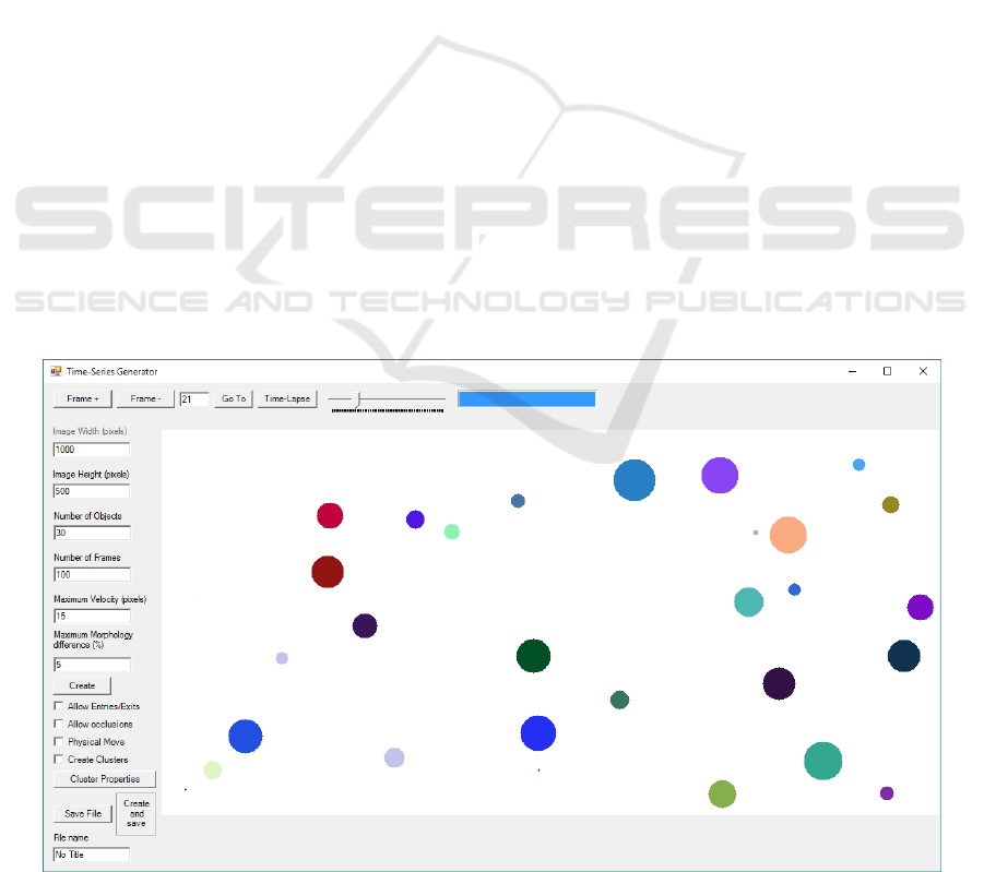
The tool interface is shown in Figure 1. At the

top row of the window there are frame handlers, to

advance forward and backward in the time-series, or

to go directly to a specific frame. The “Time-Lapse”

button reproduces the full time-series, one frame per

40 milliseconds.

The left bar contains the boxes to write the

desired width and height of images, in pixels. Then

the user can choose the number of objects in each

frame, and the total number of frames. The

“Maximum Velocity” is the maximum distance, in

pixels, that an object can travel between frames,

while the “Maximum Morphology Difference” is the

maximum difference of the “morphology” factor

that an object can have between frames, in

percentage. The “Physical Move” button controls the

option of giving objects physical limitations to their

kinetics. If it is selected, each object has a velocity

and orientation assigned to it, meaning that its

position dynamics will depend on these two

variables. If it is not selected, objects will move

arbitrarily between frames.

One can also select “Allow Entries/Exits”, to

allow the objects to enter and exit the image limits.

If unselected, objects collide with the edges of the

image when reaching them.

Overlapping of cells is possible, using the

“Allow Occlusions” option. When this option is

selected, objects move without restrictions due to

superposition between them. If it is not selected,

objects will collide between them similarly as when

colliding with the edges.

One can also force the objects to organize into

clusters, by checking the “Create Clusters” option.

When selected, all objects of each cluster have the

same physical features. In this setting, “Physical

Move” is automatically selected and “Allow

Occlusions” is deselected, blocking the

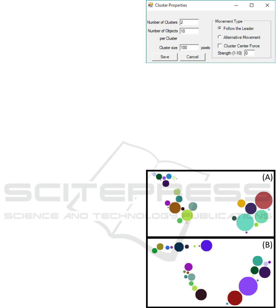
correspondent checkboxes. The button “Cluster

Properties” (shown in Figure 2) leads to a new

window with the options for clusters’ creation. Here,

one can choose the desired number of clusters, the

number of objects per cluster, and the size of the

clusters in pixels. It is also possible to choose

between two types of objects’ kinetics: “Follow the

Leader” and “Alternative Movement”. The

application of “Cluster Centre Force” and its

strength are shown in Figure 3 and explained in

Section 3.2.2.

3.2 Object Modelling

This sub-section focuses on the modelled features,

Figure 1: Image Generator Tool interface.

SIMULTECH 2016 - 6th International Conference on Simulation and Modeling Methodologies, Technologies and Applications

namely object movement and cluster, based on

biologically inspired objects, such as bacteria cells.

3.2.1 Object Motility

According to the user’s selection, objects can have

movement respecting a number of physical rules. If

this option is deactivated, objects will move

arbitrarily through the image.

Objects in each frame are only represented by

their position in coordinates in x and y and their

morphology factor. In each frame, each object can

move to a new x and y coordinates by an arbitrary

distance that cannot be higher than the “Maximum

Velocity” value in pixels.

With occlusions and “exits and entries” also

deactivated, objects will avoid the positions where

they collide with other objects or go out the image

boundaries, searching for a position considering

these limitations and the maximum distance they can

move between frames.

If the user chooses to give objects “Physical

Move”, in addition to previous features, each object

will have a velocity and an orientation (physical

parameters) assigned to it, meaning that their

position dynamics will depend on these two values.

In each frame, each object will have new x and y

coordinates distanced “d” (no bigger than

“Maximum Velocity”) from the previous frame

coordinates, direction “o” (between 0 and 2pi

radians), with both components using an

independent random variable.

If entries and exits are deactivated and if an

object is heading to the image boundary, it is

reflected respecting Snell’s Law, causing a change

in the angle’s direction of movement. If occlusions

are deactivated, when two objects are about to

collide, they change to opposite orientations in an

approximation to the reflection laws, but ignoring

differences in their morphologies.

3.2.2 Cluster Creation

When selecting the option “Create Clusters”, the

Generator will create a time-series with the number

of clusters, objects and size of cluster chosen by the

user.

These options (shown in Figure 2) must be

consistent and take into consideration the image

size.

In “Alternative Movement” (as shown in Figure

3-A) all objects of each cluster have the same

physical parameters, which means that they move in

the same direction with the same speed (with a small

independent arbitrary component).

Figure 2: Interface options for cluster properties.

In the “Follow the Leader” movement mode (as

shown in Figure 3-B), each cluster has a leading

object. The characteristics of the other objects of the

same cluster are dependent on the leader’s

behaviour. The leader “receives” the physical

parameters at first frame (velocity and orientation)

and at each frame the other objects of its cluster will

move in the leader’s direction, minimizing the

distance to it, but respecting the “non-collision” rule.

If two objects from different clusters collide, one of

them will start belonging to the other cluster. This

may cause the “merging” of clusters.

Figure 3: Exemplificative frames of (a) ‘Alternative’

Movement (b) ‘Follow the leader’ Movement.

The “Cluster Centre Force” feature is exclusively

for “Alternative Movement” that creates an

attraction force at the cluster’s centre, with a

selectable strength selected by the user. This force

keeps cluster’s objects together, even when colliding

with the image borders or other objects. Increasing

the strength, the objects will move faster to the

An Image Generator Platform to Improve Cell Tracking Algorithms - Simulation of Objects of Various Morphologies, Kinetics and

Clustering

cluster’s centre. In this mode of motility, when

objects from different clusters collide, they will be

“left behind” by their cluster until they can join it

again.

3.3 Tested Tracking Algorithms

3.3.1 Simple Nearest-Neighbour Algorithm

The first tracking algorithm tested was the Simple

Nearest-Neighbour (NN). This method only takes

into consideration the position of each object in each

frame of the time-series, and uses the Euclidian

Distance between points to find matching objects

between frame n and n+1. Being 



the distance

between two objects:







































(1)

Where 



and 



are the positions of each object in

frame n and 



and 



are the positions in frame

n+1. Having the distance between each object in

frame n and all objects in frame n+1,

correspondences are made based on the minimum

distance. The object in frame n+1 closer to each

object in frame n is assigned to it. If two objects in

n+1 are assigned to the same object in n, the closer

object is assigned, until all correspondences between

frames are unique (Elfring et al., 2010).

3.3.2 Nearest-Neighbour with Morphology

Algorithm

The next algorithm tested was the Nearest

Neighbour with Morphology (NNm). This method

accounts not only for the differences between the

positions of each object in each frame, but also for a

shape-related factor, called morphology.

This algorithm calculates the distance percolated

by each object between frames n and n+1 using

equation (1). Being 



the morphology of each

object in frame n, and 



the shape factor in n+1,

the difference, 



, between these variables is

calculated by:















(2)

The total difference,



, between each object in

each frame pair is given by (3) with  and  being

the weights given to each partial distance.





∙



∙



(3)

Here different weights are used (as presented in the

Results section), in order to study the best way to

combine them, to achieve the best possible results.

3.3.3 Cluster Tracking

Identifying clusters is one of the most complex

issues of image characterization (Czink et al., 2006).

In this work, the problem lays in tracking objects

knowing that they are grouped in clusters. Bacteria

often group in this way, so the goal is to find a

method that improves tracking of clustered objects.

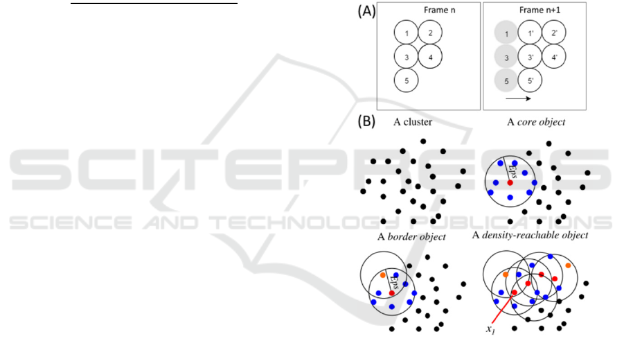
One of the main problems of clustered objects is

illustrated in Figure 4-A. Using Nearest-Neighbour

(or Nearest Neighbour with Morphology) to track

these frames, the algorithm will immediately

misidentify at least two of the objects of frame n+1.

This will occur in objects 1’ and 3’, and it happens

because their position in n+1 is exactly the same that

objects 2 and 4 have in n.

Figure 4: (A) Example of a possible misidentification

using the Nearest-Neighbour Algorithms. (B) After

defining ‘MinPts’ as the minimal number of objects in the

neighbourhood, and Eps as the neighbourhood radius, we

can define a core object (Red) when its local density is

higher than ‘MinPts’ and a border object (Orange) if its

local density is less than ‘MinPts’. Two density-reachable

objects are defined if there exists a chain of core objects

with distances between them smaller than Eps. Adapted

from (Tran et al., 2013).

To solve this problem we choose to implement a

novel tracking algorithm that considers the cluster’s

features and singularities. The developed method to

track clustered objects has several steps, and the first

is to correctly identify the clusters and objects

belonging to them. The method is called Density-

SIMULTECH 2016 - 6th International Conference on Simulation and Modeling Methodologies, Technologies and Applications

Based Spatial Clustering of Applications with Noise

(DBSCAN) (Ester et al., 1996) in its revised version

(Tran et al., 2013). This method formalizes the

notion of “cluster” and “noise”, using the definition

of density to characterize clusters, which means that

to define a cluster, the density of the neighbourhood

of each point has to be higher than a given threshold.

‘MinPts’ are the minimal number of objects in the

neighbourhood, and Eps is the neighbourhood radius

(see figure 4-B).

Objects can be divided in three categories: core,

border and noise (see figure 4-B). An object is a core

object if its local density is higher than ‘MinPts’. It

is considered a border object if its local density is

less than ‘MinPts’ and it belongs to the

neighbourhood of a core object. An object is

classified as a noise if in its Eps radius there are less

than ‘MinPts’ objects and none is a core.

Finally, we identify two density-reachable

objects if there exists a chain of core objects

between them (see Figure 4-B), with distances

between them smaller than ‘MinPts’ (Tran et al.,

2013).

This approach improves clustering identification

when data has dense adjacent clusters (Tran et al.,,

2013). They also introduced the core-density-

reachable objects, which are the same as the chain of

density-reachable objects, but cutting border objects

from chain’s ends and staying unclassified until all

core objects are identified (Tran et al., 2013).

The algorithm has two main steps: ‘dbscan’ and

‘ExpandCluster’. The first step lies in covering each

object and running ‘ExpandCluster’ if the object is

unclassified. Then, it returns all objects that are

core-density-reachable from that one. If it is a core

object, a cluster is produced. If it is a border object,

it has no core-density-reachable objects, and follows

to the next one. After all chains from the core object

are known, it is assigned to its best density-reachable

chain and all border objects.

After identifying the clusters in all frames with

DBSCAN, a novel algorithm for object tracking was

developed. This algorithm assumes that objects are

grouped and move in clusters, treating each cluster

as a separate individual while tracking. The first step

(with all clusters identified) is to isolate the clusters

and calculate their centroid, in coordinates x and y:







∑













(4)

After all centroids are calculated, they are processed

as objects, since they have their own coordinates.

The Nearest-Neighbour algorithm is then applied to

these coordinates, tracking the clusters and resulting

in a sequence of results similar to object tracking but

treating a cluster individually.

4 RESULTS AND DISCUSSION

We generated several time-series that can be used as

a benchmark to test tracking algorithms. For this, we

simulated examples with different starting number

of objects (20 to 160) and ‘Maximum Velocity’

(V=5, 10, 15, 20 and 30).

The generated images have a 1000x500 pixel

size (first and second experiment) and 1500x100

(third experiment). The implemented Tracking

Algorithms automatically processes the csv files

with the objects’ true positions produced by the

Image Generator. The detected object tracking is

then compared with the gold standard, where one

error is counted when one object is incorrectly

tracked from one frame to another it is considered a

False Positive (FP). When one object is tracked

correctly between two consecutive frames it is

considered a True Positive (TP). It is important to

notice that errors that occur in the beginning of the

time series are typically propagated through the

entire sequence. We present in the following tables

the tracking errors (false discovery rate), calculated

as FP/(FP+TP).

4.1 Simple Nearest-Neighbour

Algorithm

We tested 10 time-series of 100 frames for each

example with different objects and different

maximum velocity. In Table 1, we present the

tracking performance of the Simple Nearest-

Neighbour Algorithm, based on the ground-truth

produced by the image generator. A tracking error is

calculated on every frame and accumulated to the

end of the time-series.

Table 1: Tracking errors of the Simple Nearest-Neighbour

Algorithm.

Obj. V=5 V=10 V=15 V=20 V=30

20 0,00 0,92 1,06 4,19 19,20

40 0,26 1,27 3,23 5,93 24,01

60 0,06 1,58 5,63 12,38 39,66

80 0,24 1,84 6,62 15,74 45,06

100 0,27 1,20 7,85 19,94 49,76

120 0,22 1,69 10,57 21,16 51,86

140 0,55 3,71 14,16 26,57 58,07

160 0,42 4,12 14,91 33,74 63,89

An Image Generator Platform to Improve Cell Tracking Algorithms - Simulation of Objects of Various Morphologies, Kinetics and

Clustering

In this case, the morphology shape-related factor

called was set at 0.05 (this value was chosen to

emulate biologically inspired objects that slowly

change their shape over time).

The results from Table 1 show that this simple

algorithm can still handle the increase in the number

of objects while keeping a small velocity, and that

increasing the velocity from 15 to 20 and 30 the

tracking performance was significantly reduced.

4.2 Nearest-Neighbour with

Morphology Algorithm

In this second experiment, we show how tracking

taking into account the morphology of the object can

be helpful in the worst case scenario of the last

experiment. In Table 2, we present the results of the

tracking performance of the Nearest-Neighbour with

Morphology Algorithm.

In this case we also produced 10 time-series of

100 frames for each example with different objects

and different maximum velocity, but also with

distinct morphology factors.

We tested the algorithm in two configurations;

the first giving a 60% importance to the calculated

distance between objects ( factor in equation 3) and

40% to the calculated morphology difference (

factor). For the second configuration we used 40%

for  and 60% for . Here we also changed the

shape-related factor and used both 0.05 and 0.1

values.

Table 2: Tracking errors of the Nearest-Neighbour with

Morphology Algorithm.

 = 60% and =40%

m factor= 0.05 m factor= 0.1

Obj. V=15 V=20 V=30 V=15 V=20 V=30

100 6,02 14,71 41,60 6,03 17,79 40,55

120 6,27 14,92 42,05 9,24 19,68 44,45

140 9,29 18,34 48,96 8,34 21,59 48,90

160 10,32 25,49 55,35 10,26 25,39 55,32

Obj.

 = 40% and =60%

100 4,26 10,57 33,37 3,96 12,07 32,44

120 4,53 10,80 33,95 6,39 14,07 37,09

140 6,36 14,58 39,30 5,34 15,18 41,36

160 7,27 20,78 46,81 8,06 18,93 49,38

From Table 2, we observe that tracking results

can be improved by using the Morphology

Algorithm (e.g. in the worst case scenario the error

percentage was reduced from 64% to 47%).

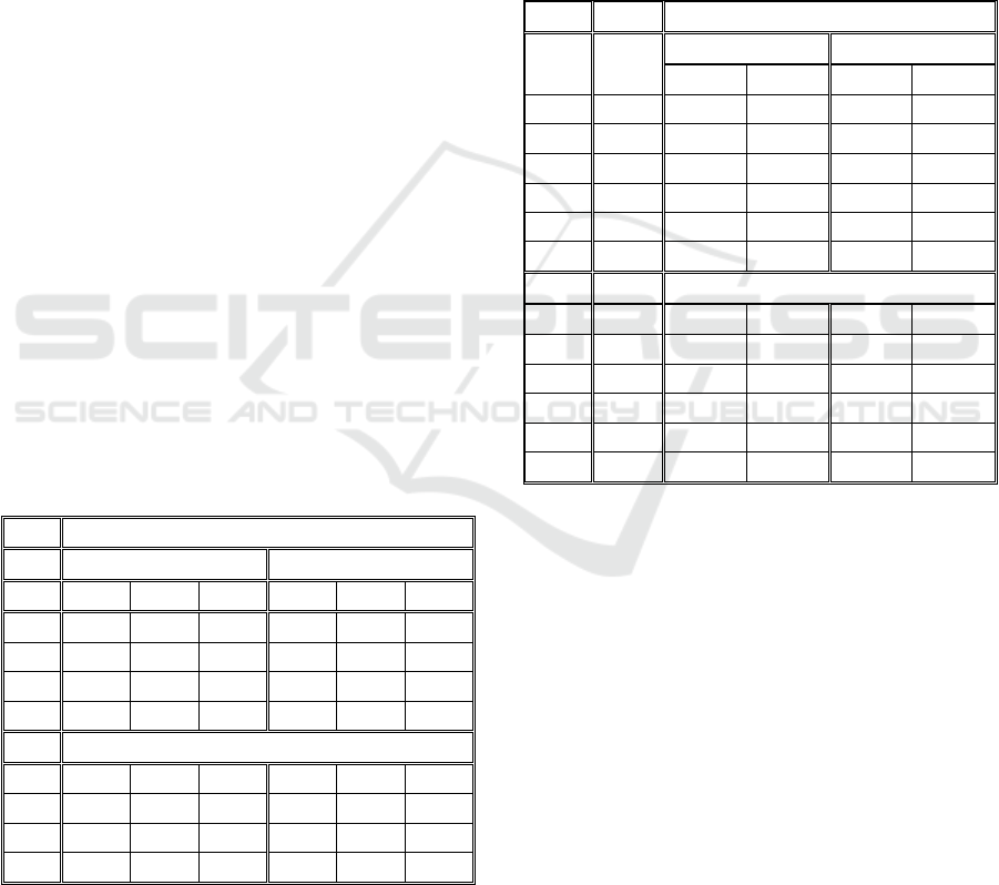
4.3 Cluster Tracking

The Create Clusters property was used to test the

same tracking algorithms (Simple NN and NN with

Morphology Algorithms with  = 40%). The

simulated parameters were: number of clusters (1, 5

or 10), number of objects per cluster (10 or 15),

maximum velocity (5 or 10), Alternative Movement,

Center Force (4) and morphology factor (0 or 0.05).

The tracking results are presented in table 3.

Table 3: Tracking errors, within clusters with different

properties, using the Simple and Morphology Nearest-

Neighbour Algorithms.

Simple NN Algorithm

Nº of

Clust

Obj. /

Clust.

m factor= 0 m factor= 0.05

V=5 V=10 V=5 V=10

1 10 7,79 30,42 9,88 23,33

1 15 11,74 50,91 10,74 38,06

5 10 7,48 34,71 10,95 31,89

5 15 17,43 45,22 16,06 44,51

10 10 12,20 38,26 11,64 42,47

10 15 21,14 53,90 23,52 57,34

NN with Morphology

1 10 1,27 4,879 5,52 13,83

1 15 3,76 21,15 4,63 20,76

5 10 1,80 12,98 4,69 15,93

5 15 7,16 20,77 5,94 22,07

10 10 3,78 16,15 4,55 19,71

10 15 8,73 28,36 10,13 34,12

For the Cluster creation, we used 10 time-series

(and averaged the results) of 200 frames and

calculated the object tracking on every frame and

accumulated to the end of the time-series.

The DBSCAN algorithm tries to separate each

cluster in every frame. Therefore, if the number of

clusters is the same between the actual frame and the

previous one (t and t-1), then they are matched using

NN, treating them as isolated objects and aligned

using their centroids. If the number of clusters

changes, we skip the first step and check the number

of objects inside each cluster. When there are more

objects in t then in t-1, these ‘extra’ objects are

called ‘Possible Entry’, if there are less objects, they

are called ‘Possible Exit’.

This classification is done temporarily and

compares the "Possible Exit" features to the features

of all other objects of the frame t-1, linking it to a

"Possible entry" in another cluster (meaning that it

left one cluster to join another), classifying it as

SIMULTECH 2016 - 6th International Conference on Simulation and Modeling Methodologies, Technologies and Applications

noise, or as an object leaving the image. The main

difference between the two DBSCAN Algorithms is

that, in the first, this classification is done after the

tracking and in the second it is done before the

tracking, equalizing the number of objects between

the clusters.

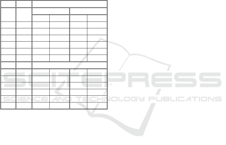
Results from both DBSCAN Algorithms are

presented in Table 4. We can see that DBSCAN

Algorithms do not improve significantly over the

Nearest-Neighbour with Morphology.

Table 4: Tracking errors, within clusters with different

properties, using two different DBSCAN Algorithms.

DBSCAN 1

Nº of

Clust

Obj. /

Clust.

m factor= 0 m factor= 0.05

V=5 V=10 V=5 V=10

1 10 5,55 2,97 9,64 9,14

1 15 1,92 12,94 3,87 10,49

5 10 5,43 13,71 6,42 16,61

5 15 5,84 19,29 6,49 20,84

10 10 5,81 17,55 6,42 21,07

10 15 8,65 28,29 9,91 34,52

DBSCAN 2

1 10 4,67 2,97 9,64 7,82

1 15 2,59 12,96 3,87 10,49

5 10 5,54 14,56 7,55 17,37

5 15 5,74 19,35 6,19 20,82

10 10 6,00 17,57 6,43 21,42

10 15 8,65 28,29 9,98 34,52

A strange behaviour with just 1 cluster was

identified in the DBSCAN algorithms, where

increasing the objects actually decreased the

tracking errors. This behaviour could be due to a

bigger movement restriction within clusters with

higher objects, but further studies are required to

analyse this behaviour.

5 CONCLUSIONS AND FUTURE

WORK

To support high-throughput experiments of single

cell imaging, reliable automated image processing

methods are required. Although most studies focus

on automatic segmentation of cells or cellular

structures, in a time-series a proper object tracking is

also necessary, particularly since errors in tracking

are propagated, meaning that even small tracking

errors (particularly on the initial frames) can lead to

a high percentage of misidentified tracks.

To validate such Tracking Algorithms, it is

necessary to use a labelled ‘ground truth’.

Sometimes this ground-truth is manually processed,

which can be unfeasible in a Big Data scenario. A

more viable alternative is to generate artificial

images by simulating biological cell models. To

produce such artificial images we developed an open

source platform that can simulate biologically

inspired bacterial systems, by creating cells with

different morphologies, physical movement and

cluster creation. Using this Platform, we evaluated

three tracking algorithms (Simple Nearest-

Neighbour, Nearest-Neighbour with Morphology

and two variations of the DBSCAN Algorithm).

The obtained results showed that, for cases with

lower maximum velocity, the Simple Nearest-

Neighbour Algorithm was able to track objects even

with a significant increase in the number of objects.

The Nearest-Neighbour with Morphology algorithm

can help in reducing tracking errors when the

velocity is increased. In the example where we

forced the creation of clusters, both the Nearest-

Neighbour with Morphology and the DBSCAN

algorithms showed similar results. In the near future,

we plan to study and compare other tracking

methodologies in different cluster configurations.

We expect this open-sourced tool (available at:

http://griduni.uninova.pt/Clustergen/

ClusterGen_v1.0.zip) to help future endeavours in

the development of new tracking algorithms, as it

can produce huge amount of benchmarked data in

various configurations.

Future developments of this tool involve adding

an object division module, which can be used to test

division tracking in dense clusters. We also plan to

add a module that introduces secondary bodies

inside the primary objects, simulating internal cell

organelles and structures. A future application will

also be made available as a web-based system to

improve usability and compatibility.

ACKNOWLEGMENTS

Work supported by the Portuguese Foundation for

Science and Technology (FCT/MCTES) through a

PhD Scholarship, ref. SFRH/BD/88987/2012 to LM,

SADAC project (ref. PTDC/BBB-MET/1084/2012)

and by FCT Strategic Program UID/EEA/00066/203

of UNINOVA, CTS. This work is also funded by the

Academy of Finland [ref. 126803 to ASR].

An Image Generator Platform to Improve Cell Tracking Algorithms - Simulation of Objects of Various Morphologies, Kinetics and

Clustering

REFERENCES

Bhattacharyya, A., 1943. On a Measure of Divergence

Between Two Statistical Populations Defined by

Probability Distributions. Bulletin of the Calcutta

Mathematical Society, 35, pp.99–110.

Bonnet, N., 2004. Some trends in microscope image

processing. Micron (Oxford, England : 1993), 35(8),

pp.635–653.

Coelho, L.P., Shariff, A. & Murphy, R.F., 2009. Nuclear

Segmentation In Microscope Cell Images A Hand-

Segmented Dataset And Comparison Of Algorithms.

In Proc IEEE Int Symp Biomed Imaging. pp. 518–521.

Coutu, D.L. & Schroeder, T., 2013. Probing cellular

processes by long-term live imaging--historic

problems and current solutions. Journal of cell

science, 126(Pt 17), pp.3805–15.

Czink, N., Mecklenbräuker, C. & Del Galdo, G., 2006. A

novel automatic cluster tracking algorithm. IEEE

International Symposium on Personal, Indoor and

Mobile Radio Communications, PIMRC, pp.1–5.

Danuser, G., 2011. Computer vision in cell biology. Cell,

147(5), pp.973–8.

Deshmukh, M. & Bhosle, U., 2011. A survey of image

registration. International Journal of Image

Processing, 5(3), pp.245–269.

Elfring, J., Janssen, R. & van de Molengraft, R., 2010.

Data Association and Tracking: A Literature Survey.

In ICT Call 4 RoboEarth Project.

Ester, M. et al., 1996. A Density-Based Algorithm for

Discovering Clusters in Large Spatial Databases with

Noise. In 2nd Int. Conference on Knowledge

Discovery and Data Mining. pp. 226–231.

Frigault, M. et al., 2009. Live-cell microscopy - tips and

tools. Journal of Cell Science, 122(6), pp.753–767.

Gorji, A. & Menhaj, M.B., 2007. Multiple Target

Tracking for Mobile Robots Using the JPDAF

Algorithm. In 19th IEEE International Conference on

Tools with Artificial Intelligence (ICTAI 2007). pp.

137–145.

Gotelli, N.J. & McGill, B.J., 1996. Null versus neutral

models: what’s the difference? Ecography, 29(5),

pp.793–800.

Gu, S., Zheng, Y. & Tomasi, C., 2011. Efficient visual

object tracking with online nearest neighbor classifier.

In Computer Vision – ACCV 2010. Volume 6492 of the

series LNCS. pp. 271–282.

Häkkinen, A. et al., 2013. CellAging: a tool to study

segregation and partitioning in division in cell lineages

of Escherichia coli. Bioinformatics (Oxford, England),

29(13), pp.1708–1709.

Joyce, J., 2014. Kullback-Leibler Divergence. In M.

Lovric, ed. International Encyclopedia of Statistical

Science SE - 327. Springer Berlin Heidelberg, pp.

720–722.

Kruse, K., 2012. Bacterial Organization in Space and

Time. In Comprehensive Biophysics. pp. 208–221.

Lehmussola, A. et al., 2007. Computational framework for

simulating fluorescence microscope images with cell

populations. IEEE transactions on medical imaging,

26(7), pp.1010–6.

Lehmussola, A. et al., 2011. Synthetic Images of High-

Throughput Microscopy for Validation of Image

Analysis Methods. Proceedings of the IEEE, 96(8),

pp.1348 – 1360.

Martins, L., Fonseca, J. & Ribeiro, A., 2015. “miSimBa” -

A simulator of synthetic time-lapsed microscopy

images of bacterial cells. In Proceedings - 2015 IEEE

4th Portuguese Meeting on Bioengineering, ENBENG

2015. pp. 1 – 6.

Meijering, E., 2012. Cell Segmentation: 50 Years Down

the Road. IEEE Signal Processing Magazine, 29(5),

pp.140–145.

Misteli, T., 2007. Beyond the sequence: cellular

organization of genome function. Cell, 128(4),

pp.787–800.

Murphy, R., 2012. CellOrganizer: Image-derived Models

of Subcellular Organization and Protein Distribution.

Methods in Cell Biology, 110, pp.179–93.

Ruusuvuori, P. et al., 2008. Benchmark Set Of Synthetic

Images For Validating Cell Image Analysis

Algorithms. In Proceedings of the 16th European

Signal Processing Conference, EUSIPCO.

Satwik, R. et al., 2012. SimuCell : a flexible framework

for creating synthetic microscopy images a

PhenoRipper : software for rapidly profiling

microscopy images. , 9(7), pp.634–636.

Selinummi, J. et al., 2005. Software for quantification of

labeled bacteria from digital microscope images by

automated image analysis. BioTechniques, 39(6),

pp.859–863.

Shi, J. & Tomasi, C., 1994. Good features to track. In

Proceedings CVPR’94. 1994 IEEE Computer Society

Conference on. IEEE. pp. 593–600.

Sliusarenko, O. & Heinritz, J., 2011. High-throughput,

subpixel precision analysis of bacterial morphogenesis

and intracellular spatio-temporal dynamics. Molecular

Microbiology, 80(3), pp.612–627.

Smith, A., 1993. Novel approach to nonlinear/non-

Gaussian Bayesian state estimation. Radar and Signal

Processing, IEE Proceedings F, 140(2), pp.107–113.

Sung, M.-H. & McNally, J.G., 2011. Live cell imaging

and systems biology. Wiley interdisciplinary reviews.

Systems biology and medicine, 3(2), pp.167–82.

Svoboda, D. et al., 2007. On simulating 3D Fluorescent

Microscope Images. In Computer Analysis of Images

and Patterns -12th International Conference, CAIP

2007, Vienna, Austria, August 27-29, 2007.

Proceedings. pp. 309–316.

Svoboda, D., Kozubek, M. & Stejskal, S., 2009.

Generation of digital phantoms of cell nuclei and

simulation of image formation in 3D image cytometry.

Cytometry. Part A : the journal of the International

Society for Analytical Cytology, 75(6), pp.494–509.

Tissainayagam, P. & Suter, D., 2005. Object tracking in

image sequences using point features. Pattern

Recognition

, 38(1), pp.105–113.

Tran, T.N., Drab, K. & Daszykowski, M., 2013. Revised

DBSCAN algorithm to cluster data with dense

SIMULTECH 2016 - 6th International Conference on Simulation and Modeling Methodologies, Technologies and Applications

adjacent clusters. Chemometrics and Intelligent

Laboratory Systems, 120, pp.92–96.

Ulman, V., Oremus, Z. & Svoboda, D., 2015. TRAgen: A

Tool for Generation of Synthetic Time-Lapse Image

Sequences of Living Cells. In Proceedings of 18th

International Conference on Image Analysis and

Processing (ICIAP 2015). Springer International

Publishing, pp. 623–634.

Wang, Q. et al., 2010. Image segmentation and dynamic

lineage analysis in single-cell fluorescence

microscopy. Cytometry A, 77(1), pp.101–110.

Wyawahare, M., Patil, P. & Abhyankar, H., 2009. Image

Registration Techniques : An overview. Int. Journal of

Signal Processing, Image Processing and Pattern

Recognition, 2(3), pp.11–28.

Xiong, W. et al., 2010. Learning Cell Geometry Models

For Cell Image Simulation : An Unbiased Approach.

In Proceedings of 2010 IEEE 17th International

Conference on Image Processing. pp. 1897–1900.

Yilmaz, A., Javed, O. & Shah, M., 2006. Object tracking:

A survey. ACM Computing Surveys, 38(4, Article 13),

pp.1–45.

Young, J. et al., 2012. Measuring single-cell gene

expression dynamics in bacteria using fluorescence

time-lapse microscopy. Nat. Protoc., 7(1), pp.80–8.

Zhao, T. & Murphy, R.F., 2007. Automated learning of

generative models for subcellular location: building

blocks for systems biology. Cytometry. Part A : the

journal of the International Society for Analytical

Cytology, 71(12), pp.978–90.

Zhou, H., Yuan, Y. & Shi, C., 2009. Object tracking using

SIFT features and mean shift. Computer Vision and

Image Understanding, 113(3), pp.345–352.

An Image Generator Platform to Improve Cell Tracking Algorithms - Simulation of Objects of Various Morphologies, Kinetics and

Clustering