Two View Geometry Estimation by Determinant Minimization
Lorenzo Sorgi and Andrey Bushnevskiy
Technicolor Research & Innovation, Karl-Wiechert Allee 74, Hannover, Germany
Keywords:
Two View Geometry, Epipolar Geometry, Perturbation Theorem, Determinant Minimization, Tetrahedron.
Abstract:
Two view geometry estimation, the task of inferring the relative pose between two cameras using only the
image content, is one of the fundamental and most studied problems in Computer Vision. In this paper we
present a new approach for two view geometry estimation, based on the minimization of an objective function
given by the overall volume of the tetrahedrons identified in 3D space by pairs of corresponding feature
points. This error measure is equivalent to the determinant of a real valued square matrix, function of the point
match coordinates in the camera space, and we show how to minimize it taking advantage of the Perturbation
Theorem. Test performed on synthetic and real dataset confirm an increased estimation accuracy compared to
the state-of-art.
1 INTRODUCTION
Given a point in one image, is it possible to constraint
the position of the corresponding point in a second
image? The answer to this question leads to the defi-
nition of one of fundamental theorems of the geome-
try of multiple views, the Epipolar Constraint, repre-
sented with a 3x3 matrix denoted as Essential Matrix
E. This is a non invertible matrix of rank 2, indepen-
dent of a scene structure completely constrained by
the relative pose between the cameras. If a point X
in 3-space is imaged as x and x
0
in two views, then
one can show that these points satisfy the relation
hx
0
,Exi = 0, where ha,bi represents the vector inner
product. This relation was first published in 1981 by
Longuet-Higgins (Longuet-Higgins, 1987), who has
introduced the concept of Epipolar Constraint to the
computer vision community.
The first solution to the problem of Essential Ma-
trix estimation from the image correspondences was
originally proposed by Kruppa (Kruppa, 1913), where
it has been shown, that given enough correspondences
between two perspective views is possible to retrieve
all the possible configurations of the cameras, which
constitute a set of 11 solutions, among which only 10
are physically valid (Faugeras and Maybank, 1990).
Most of the techniques currently used in 3D vision
systems work with a closed-form high-order (13th
- 10th) uni-variate polynomial equation, which en-
codes the solution (Nist
´
er, 2004; Triggs, 2000; Philip,
1996). However, fifth-degree and higher-degree poly-
nomials do not have a general solution according to
the Abel-Ruffini theorem. Therefore, application of
the iterative numerical routines is required, and the
solution turns out to be highly unstable due to the in-
trinsic ill-conditioned nature of the root finding prob-
lem.
A slightly different approach, has been proposed
by Batra and al. (Batra et al., 2007), where the task of
Essential matrix estimation is reformulated as a con-
straint quadratic optimization problem, by introduc-
ing two additional constraints. In this way the authors
overcome the issue of finding the root of high degree
polynomials, but they have to tackle the problem in
an iterative way using multiple solution seeds as start-
ing point for the minimization step. With regards to
this aspect still remains open the issue how many seed
points in the solution space are required and how to
sample them.
In this paper we observe, that each pair of corre-
sponding features describes in 3D space is a tetrahe-
dron, which has a null-volume in case of correctly es-
timated camera poses. Following this observation one
can reformulate the two view geometry estimation
problem as a minimization of the cumulative volume
of the tetrahedrons defined by a set of point matches.
We will show that this is equivalent to the task of min-
imization of the sum of the determinants of a set of
square matrices, which can be solved by means of the
Perturbation Theorem (Nakatsukasa, 2011).
590
Sorgi, L. and Bushnevskiy, A.
Two View Geometry Estimation by Determinant Minimization.
DOI: 10.5220/0005677405900594
In Proceedings of the 11th Joint Conference on Computer Vision, Imaging and Computer Graphics Theory and Applications (VISIGRAPP 2016) - Volume 3: VISAPP, pages 590-594
ISBN: 978-989-758-175-5
Copyright
c
 2020 by SCITEPRESS – Science and Technology Publications, Lda. All rights reserved

2 EIGENSYSTEM
PERTURBATION
In this section we introduce the perturbation theorem
and describe its exploitation as solver for the matrix
determinant minimization. This will provide the ba-
sic mathematical tool for the solution of the two view
geometry estimation.
Let A and D be N-by-N symmetric real-valued
matrices and {λ
i
,~u
i
}
i=1...N
the eigensystem of A, that
is the set of eigenvalues and eigenvectors such that:



A~u
i
= λ
i
~u
i
~u
T
i
~u
j
= δ
i, j
A =
∑
i
λ
i
~u
i
~u
T
i
, (1)
and δ
i, j
is the Kronecker Delta-function
δ
i, j
=

1 i = j
0 i 6= j
. (2)
Considering a perturbed matrix A
0
= A + εD, for a
small ε, let {λ
0
i
,
~
u
0
i
}
i=1...N
be the eigensystem of A
0
,
corresponding to {λ
i
,~u
i
}
i=1...N
. Then the following
relations hold:





λ
0
i
= λ
i
+ ε(~u
i
· D~u
i
) + O(ε
2
)
~u
0
i
=~u
i
+ ε
∑
j6=i
(~u
j
·D~u
i
)~u
j
λ
i
−λ
j
+ O(ε
2
)
. (3)
Equations (3) are known as Perturbation Theorem.
2.1 Determinant of Perturbed Matrix
The Perturbation Theorem provides also a representa-
tion of a first order Taylor expansion of the eigensys-
tem of a A(x), denoted with {λ
i
(x),~u
i
(x)}
i=1...N
. Let
us consider a matrix function A(x) : R → S
N×N
, where
S
N×N
is the space of N-by-N symmetric positive-
definite matrices, and its first order Taylor expansion
given by
A(x + ε)
∼
=
A(x) + J
A
(x)ε + O(ε
2
), (4)
where J
A
(x) =
∂A(x)
∂x
is the Jacobian matrix of A. Sim-
ilarly the first order Taylor expansion of the corre-
sponding eigensystem can be written as

λ
i
(x + ε) = λ
i
(x) + J
λ
i
(x)ε + O(ε
2
)
~u
i
(x + ε) = ~u
i
(x) + J
u
i
(x)ε + O(ε
2
)
. (5)
Equations (5) provide the eigensystem of a matrix
A(x) affected by a small perturbation J
A
(x)ε, there-
fore the Perturbation Theorem implies that:





J
λ
i
(x) = ~u
i
(x) · J
A
(x)~u
i
J
u
i
(x) =
∑
i6= j
(~u
j
·J
A
(x)~u
i
)~u
j
λ
i
(x)−λ
j
(x)
. (6)
We recall that the determinant of the matrix A(x) is
given by the product of its eigenvalues counted with
their algebraic multiplicities. By using equations (5)
one can express the determinant of the perturbed ma-
trix as
detA(x+ε) =
∏
i
λ
i
(x+ε)
∼
=
∏
i
(λ
i
(x)+J
λ
i
(x)ε) (7)
By expanding equation (7) and neglecting the high or-
der terms in ε, one obtains
detA(x + ε) =
∏
i
λ
i
(x) +
∏
i
(
∏
j6=i
λ
j
(x))J
λ
i
(x)ε . (8)
Equation (8) provides the first order Taylor approxi-
mation of the determinant of the matrix A(x) and its
derivative is given by
∂detA(x)
∂x
∼
=
∏
i
(
∏
j6=i
λ
j
(x))J
λ
i
(x) (9)
An equivalent formulation can be derived also for the
determinant of a non-symmetric matrices. Let us con-
sider a D×D non-symmetric matrix M(x) and its Sin-
gular Value Decomposition
M(x) = U · Σ ·V
T
(10)
where the notation Σ is a diagonal matrix containing
on the singular values {σ
j
}
j=1,...,D
. By applying the
determinant relation det(AB) = det(A)det(B) one ob-
tains
detM(x) = detU · detΣ · detV
T
=
∏
i
σ
i
(x) (11)
Let us define the symmetric matrix K(x) = M(x) ·
M
T
(x). The singular values of the matrix M(x ) are
related to the eigenvalues λ
i
of K(x) by the expres-
sion λ
i
= σ
2
i
, therefore by differentiation we obtain
J
λ
i
= 2σ
i
· J
σ
i
(12)
As the matrix K(x) is by definition symmetric, one
can apply the results of the Perturbation Theorem to
compute the Jacobian J
λ
i
of its eigenvalues and ex-
press the first order Taylor approximation of the de-
terminant of the non-symmetric matrix M(x) as
detM(x + ε)
∼
=
detM(x) +
∏
i
(
∏
j6=i
σ
j
(x))
J
λ
i
(x)
2σ
i
(x)
ε
(13)
2.2 Two View Geometry Estimation
Let us consider a two-view geometry model in Fig.1,
where m and m
0
are projections of a 3D point M on
the image planes of two cameras.
We assume to be working in calibrated camera condi-
tion, therefore each image point m can be mapped to
Two View Geometry Estimation by Determinant Minimization
591

Figure 1: Two-view projection model in a calibrated camera
space.
the corresponding incident vectors ˆm by inverting the
cameras projection functions (Hartley and Zisserman,
2004). Without loss of generality we can assume the
projection center of the first camera to be located in
the origin of the reference system, O = [

0 0 0

]
T
.
Let us also denote with {R,t} ∈ SO(3) the Euclidean
transformation relating two camera systems, which
enables the definition of the incident vector in the sec-
ond camera system as
ˆm
0
∼ R(M − t), (14)
where ∼ denotes equality up to a non-zero scale fac-
tor.
One can easily infer that the four points
{O, ˆm,t, R
T
ˆm
0
+ t} lay on the same plane, defined by
the line OC and the point M; which is also a straight-
forward consequence of the epipolar constraint. An
alternative interpretation of the coplanarity constraint
is given in 3D if one considers a solid, namely the
tetrahedron, identified by the four points, (Fig.2(a)).
In the ideal case the latter has null volume, however
noisy image projections or incorrect 2-view geome-
try parameters lead to the construction of a non-zero
volume (Fig.2(b)).
The volume V of a tetrahedron with vertices
{a,b,c,d} can be computed from the determinant of
the matrix M
V
by the relation
V =
1
6
detM
V
, (15)
where M
V
= [(a−b), (b−c), (c−d), ] is constructed
using the vertices coordinates. Therefore by applying
the previous equation 15 to the tetrahedron in (Fig.2),
one can compute its volume as a fraction of the deter-
minant of the matrix A(R,t) defined as
A(R,t) = [− ˆm , ( ˆm − 1), −R
T
ˆm
0
] (16)
where the matrix A(R,t) is explicitly indicated as a
function of the camera motion {R,t}.
(a)
(b)
Figure 2: Tetrahedron built using corresponding feature
point in case of correctly (a) and incorrectly (b) estimated
camera pose.
This simple geometrical model allows for the for-
mulation of the 2-view geometry estimation problem,
given a set of N point correspondences between two
views, as the solution of the minimization problem
{
¯
R,
¯
t} = argmax
{R,t}∈SO(3)
∑
k=1,...,N
det
2
(A
k
(R,t)), (17)
where A
k
(R,t) is the matrix build according to the
equation (16) using the k-th point correspondence.
The objective function (17) is minimized using the
Levenberg-Marquardt algorithm and in each iteration
the normal equation is build using equations (11) and
(13) to express the error contributions and their Jaco-
bian.
3 RESULTS
The proposed technique has been evaluated on syn-
thetic and real data and compared with the standard
approach, based on the minimization of the Sampson
error (Hartley and Zisserman, 2004; Zhang, 1998).
3.1 Synthetic Data
The synthetic model was comprised of a point cloud
containing 100 randomly positioned 3D points and
two virtual cameras, randomly located at a fixed dis-
tance with the respect to the point cloud. Each camera
was modeled as a 50 horizontal field-of-view lens and
1024x768 sensor. The stereo geometry was randomly
sampled from the subspace of Euclidean Transforma-
tions {R,t}, such that
k
t
k
= 1.
The image projections of the points were cor-
rupted using a zero-mean white Gaussian noise with
increasing standard deviation ranging within the in-
terval [0, 2] pixels. For each level of image noise 50
VISAPP 2016 - International Conference on Computer Vision Theory and Applications
592

random scenes were generated and the median and
the standard deviation of the estimation errors were
collected. The rotation and translation errors are pre-
sented by two angular measures: the angle between
the estimated and real baseline vectors, and the angle
associated to the difference rotation δR between the
estimated
˜
R and real R rotations, δR = R
T
˜
R. In both
tests algorithm was initialized with the ideal stereo ge-
ometry, given by the null rotation and the unit norm
x-vector {I
3
,[1 0 0]
T
}.
(a)
(b)
Figure 3: Synthetic results. Error for estimated camera ro-
tation (a) and translation (b).
The results, presented in Fig.3. demonstrate,
that the accuracy of the proposed method is higher
than the one, based on the Sampson Error minimiza-
tion. The interesting aspect is that the convergence
of the minimization of the proposed error function is
achieved irrespective to the proximity of the initializa-
tion point to the actual solution. This does not apply
to the Sampson Error minimization approach, where a
number of trials have failed to converge to the correct
solution.
3.2 Real Data
For the real data test we have used a set images from
two GoPro Hero 3+ action cameras, set in a stereo
configuration on the planar surface Fig.4(a). The in-
trinsic parameters of the cameras were pre-estimated
using our own calibration tool, based on the calibra-
tion approach, presented in (Kanatani, 2013). The
feature points positions and their descriptors were ex-
tracted from each of two views and matched.
(a)
(b)
Figure 4: Real dataset test. Stereo camera configuration (a)
and estimated geometry (b).
In order to minimize the influence of the outliers, only
the feature correspondences, valid in both directions
were used for the geometry estimation. The recon-
structed geometry, presented in Fig.4(b) confirms the
efficiency of the proposed method.
In order to asses the quality of the stereo geome-
try recovered using the proposed approach, we have
designed a test using a black and white checkerboard
pattern. The relative geometry of two cameras has
been first estimated using the proposed method and
the feature set extracted from the snapshots of the ac-
tual scene.
A set of corresponding snapshots of a checker-
board pattern then has been taken in such a way,
that the grid has been simultaneously visible in both
views. The grid points have been detected in each
of the views, triangulated in 3D space using the es-
timated camera geometry and then projected back to
the original views. The error then has been estimated
as an average displacement between the detected and
backprojected grid points (Fig.5). The resulting back-
projection error with the mean µ = 2.9px and the stan-
dard deviation σ = 0.67px confirms the accuracy of
Two View Geometry Estimation by Determinant Minimization
593

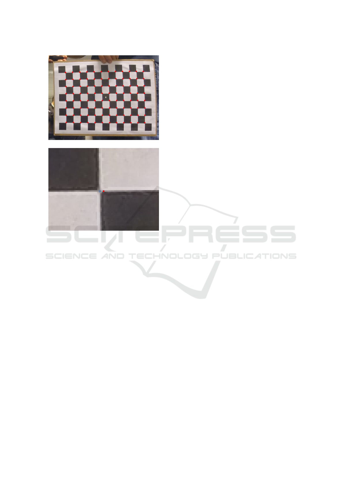
(a)
(b)
Figure 5: Real dataset test. A crop of the black and white
pattern view (a), detected (blue circle) and backprojected
(red dot) points (b).
the proposed approach and suggests the possibility
of its straightforward application without any subse-
quent refinement.
4 CONCLUSIONS
We have presented a novel approach for the two view
geometry estimation, based on the tetrahedron vol-
ume minimization using a Perturbation Theorem. The
evaluation using synthetic and real datasets and com-
parison to the standard Sampson Error minimization
algorithm confirms the accuracy of the method. The
approach features a major advantage, namely the geo-
metrical nature of the objective function, which leads
to an increase in the estimation accuracy and allows
for a very rough initialization of the numerical itera-
tions without the requirement of multiple seeds.
REFERENCES
Batra, D., Nabbe, B., and Hebert, M. (2007). An alternative
formulation for five point relative pose problem. Mo-
tion and Video Computing, IEEE Workshop on, 0:21.
Faugeras, O. D. and Maybank, S. (1990). Motion from point
matches: Multiple of solutions. Int. J. Comput. Vision,
4(3):225–246.
Hartley, R. I. and Zisserman, A. (2004). Multiple View Ge-
ometry in Computer Vision. Cambridge University
Press, ISBN: 0521540518, second edition.
Kanatani, K. (2013). Calibration of ultrawide fisheye lens
cameras by eigenvalue minimization. IEEE Trans.
Pattern Anal. Mach. Intell., 35(4):813–822.
Kruppa, E. (1913). Zur Ermittlung eines Objektes aus zwei
Perspektiven mit innerer Orientierung. H
¨
older.
Longuet-Higgins, H. C. (1987). A computer algorithm for
reconstructing a scene from two projections. In Fis-
chler, M. A. and Firschein, O., editors, Readings in
Computer Vision: Issues, Problems, Principles, and
Paradigms, pages 61–62. Kaufmann, Los Altos, CA.
Nakatsukasa, Y. (2011). Algorithms and Perturbation The-
ory for Matrix Eigenvalue Problems and the Singular
Value Decomposition. PhD thesis, Davis, CA, USA.
AAI3482268.
Nist
´
er, D. (2004). An efficient solution to the five-point rel-
ative pose problem. IEEE Trans. Pattern Anal. Mach.
Intell., 26(6):756–777.
Philip, J. (1996). A non-iterative algorithm for determining
all essential matrices corresponding to five point pairs.
The Photogrammetric Record, 15(88):589–599.
Triggs, B. (2000). Routines for relative pose of two cali-
brated cameras from 5 points. Software available from
http://lear.imag.fr/people/triggs/src.
Zhang, Z. (1998). Determining the epipolar geometry and
its uncertainty: A review. Int. J. Comput. Vision,
27(2):161–195.
VISAPP 2016 - International Conference on Computer Vision Theory and Applications
594