El MUNDO: Embedding Measurement Uncertainty in
Decision Making and Optimization
Carmen Gervet and Sylvie Galichet
LISTIC, Laboratoire d’Informatique, Systems, Traitement de l’Information et de la
Connaissance, Universit
´
e de Savoie, BP 8043974944, Annecy-Le-Vieux Cedex, France
Abstract. In this project we address the problem of modelling and solving con-
straint based problems permeated with data uncertainty, due to imprecise mea-
surements or incomplete knowledge. It is commonly specified as bounded in-
terval parameters in a constraint problem. For tractability reasons, existing ap-
proaches assume independence of the data, also called parameters. This assump-
tion is safe as no solutions are lost, but can lead to large solution spaces, and a
loss of the problem structure. In this paper we present two approaches we have
investigated in the El MUNDO project, to handle data parameter dependencies
effectively. The first one is generic whereas the second one focuses on a specific
problem structure. The first approach combines two complementary paradigms,
namely constraint programming and regression analysis, and identifies the rela-
tionships between potential solutions and parameter variations. The second ap-
proach identifies the context of matrix models and shows how dependency con-
straints over the data columns of such matrices can be modeled and handled very
efficiently. Illustrations of both approaches and their benefits are shown.
1 Introduction
Data uncertainty due to imprecise measurements or incomplete knowledge is ubiquitous
in many real world applications, such as network design, renewable energy economics,
and production planning (e.g. [16, 22]). Formalisms such as linear programming, con-
straint programming or regression analysis have been extended and successfully used
to tackle certain forms of data uncertainty. Constraint Programming (CP), is a pow-
erful paradigm used to solve decision and optimization problems in areas as diverse
as planning, scheduling, routing. The CP paradigm models a decision problem using
constraints to express the relations between variables, and propagates any information
gained from a constraint onto other constraints. When data imprecision is present, forms
of uncertainty modeling have been embedded into constraint models using bounded in-
tervals to represent such imprecise parameters, which take the form of coefficients in a
given constraint relation. The solution sought can be the most robust one, that holds un-
der the largest set of possible data realizations, or a solution set containing all solutions
under any possible realization of the data. In such problems, uncertain data dependen-
cies can exist, such as an upper bound on the sum of uncertain production rates per
machine,or the sum of traffic distribution ratios from a router over several links. To our
knowledge, existing approaches assume independence of the data when tackling real
70
Gervet C. and Galichet S.
El MUNDO: Embedding Measurement Uncertainty in Decision Making and Optimization.
DOI: 10.5220/0006162500700089
In European Project Space on Intelligent Systems, Pattern Recognition and Biomedical Systems (EPS Lisbon 2015), pages 70-89
ISBN: 978-989-758-095-6
Copyright
c
 2015 by SCITEPRESS – Science and Technology Publications, Lda. All rights reserved

world problems essentially to maintain computational tractability. This assumption is
safe in the sense that no potential solution to the uncertain problem is removed. How-
ever, the set of solutions produced can be very large even if no solution actually holds
once the data dependencies are checked. The actual structure of the problem is lost.
Thus accounting for possible data dependencies cannot be overlooked.
Fig. 1. Sigcomm4 network topology and mean values for link traffic.
Traditional models either omit any routing uncertainty for tractability reasons, and
consider solely the shortest path routing or embed the uncertain parameters but with
no dependency relationships. Values for the flow variables are derived by computing
bounded intervals, which are safe enclosing of all possible solutions. Such intervals
enclose the solution set without relating to the various instances of the parameters. For
instance, the traffic between A and C can also pass through the link A → B. Thus
the flow constraint on this link also contains 0.3..0.7 ∗ F
AC
. However, the parameter
constraint stating that the sum of the coefficients of the traffic F
AC
in both constraints
should be equal to 1 should also be present. Assuming independence of the parameters
for tractability reasons, leads to safe computations, but at the potential cost of a very
large solution set, even if no solution actually holds. No only is the problem structure
lost, but there is not insight as to how the potential solutions evolve given instances of
the data.
The question remains as to how to embed this information in a constraint model that
would remain tractable. To our knowledge this issue has not been addressed. This is the
purpose of our work.
In this paper we present two approaches to account for data dependency constraints
in decision problems. We aim to more closely model the actual problem structure, refine
the solutions produced, and add accuracy to the decision making process. The first one
uses regression analysis to identify the relationship among various instances of the un-
certain data parameters and potential solutions. Regression analysis is one of the most
widely used statistical techniques to model and represent the relationship among vari-
ables. Recently, models derived from fuzzy regression have been defined to represent
incomplete and imprecise measurements in a contextual manner, using intervals [6].
Such models apply to problems in finance or complex systems analysis in engineering
whereby a relationship between crisp or fuzzy measurements is sought.
The basic idea behind our approach is a methodological process. First we extract
the parameter constraints from the model, solve them to obtain tuple solutions over the
parameters, and run simulations on the constraint models using the parameter tuples
71
El MUNDO: Embedding Measurement Uncertainty in Decision Making and Optimization
71

as data instances that embed the dependencies. In the example above this would imply
for the two constraints given, that if one parameter takes the value 0.3, the other one
would take the value 0.7. A set of constraint models can thus be generated and solved
efficiently, matching a tuple of consistent parameters to a potential solution. Finally, we
run a regression analysis between the parameter tuples and the solutions produced to
determine the regression function, i.e. see how potential solutions relate to parameter
variations. This multidisciplinary approach is generic and provides valuable insights
to the decision maker. However, while applying it to different problems we identified a
certain problem structure that could be tackled without the need for the use of constraint
problem set.
The second approach was then designed. We identified the context of matrix mod-
els, and showed how constraints over uncertain data can be handled efficiently in this
context making powerful use of mathematical programming modeling techniques. For
instance in a production planning problem, the rows denote the products to be manu-
factured and the columns the machines available. A data constraint such as an upper
bound on the sum of uncertain production rates per machine, applies to each column of
the matrix. Matrix models are of high practical relevance in many combinatorial opti-
mization problems where the uncertain data corresponds to coefficients of the decision
variables. Clearly, the overall problem does not need to be itself a matrix model. With
the imprecise data specifying cells of an input matrix, the data constraints correspond
to restrictions over the data in each column of the matrix. In this context, we observe
that there is a dynamic relationship between the constraints over uncertain data and the
decisions variables that quantify the usage of such data. Uncertain data are not meant
to be pruned and instantiated by the decision maker. However, decision variables are
meant to be instantiated, and the solver controls their possible values. This leads us to
define a notion of relative consistency of uncertain data constraints, in relationship with
the decision variables involved, in order to reason with such constraints. For instance,
if an uncertain input does not satisfy a dependency constraint, this does not imply that
the problem has no solution! It tells us that the associated decision variable should be
0, to reflect the fact that the given machine cannot produce this input.
The main contributions of our work lies in identifying and developing two multi-
disciplinary means to study the efficient handling of uncertain data constraints. Both
approaches are novel towards the efficient handling of uncertain data constraints in
combinatorial problems. We illustrate the benefits and impacts of both approaches re-
spectively on a network flow and a production planning problem with data constraints.
The paper is structured as follows. Section 2 summarizes the related work. Section
3 describes the combination of constraint reasoning and regression analysis. Section
4 describes the concept of matrix models to handle data dependency constraints. A
conclusion is finally given in Section 5.
2 Background and Related Work
The fields of regression analysis and constraint programming are both well established
in computer science. While we identified both fields as complementary, there has been
little attempt to integrate them together to the best of our knowledge. The reason is, we
72
EPS Lisbon January 2015 2015 - European Project Space on Intelligent Systems, Pattern Recognition and Biomedical Systems
72

believe, that technology experts tackle the challenges in each research area separately.
However, each field has today reached a level of maturity shown by the dissemination in
academic and industrial works, and their integration would bring new research insights
and a novel angle in tackling real-world optimization problems with measurement un-
certainty. There has been some research in Constraint Programming (CP) to account for
data uncertainty, and similarly there has been some research in regression modeling to
use optimization techniques.
CP is a paradigm within Artificial Intelligence that proved effective and successful
to model and solve difficult combinatorial search and optimization problems from plan-
ning and resource management domains [19]. Basically it models a given problem as a
Constraint Satisfaction Problem (CSP), which means: a set of variables, the unknowns
for which we seek a value (e.g. how much to order of a given product), the range of
values allowed for each variable (e.g. the product-order variable ranges between 0 and
200), and a set of constraints which define restrictions over the variables (e.g. the prod-
uct order must be greater than 50 units). Constraint solving techniques have been pri-
marily drawn from Artificial Intelligence (constraint propagation and search), and more
recently Operations Research (graph algorithms, Linear Programming). A solution to a
constraint model is a complete consistent assignment of a value to each decision vari-
able.
In the past 15 years, the growing success of constraint programming technology
to tackle real-world combinatorial search problems, has also raised the question of its
limitations to reason with and about uncertain data, due to incomplete or imprecise mea-
surements, (e.g. energy trading, oil platform supply, scheduling). Since then the generic
CSP formalism has been extended to account for forms of uncertainty: e.g. numeri-
cal, mixed, quantified, fuzzy, uncertain CSP and CDF-interval CSPs [7]. The fuzzy and
mixed CSP [11] coined the concept of parameters, as uncontrollable variables, mean-
ing they can take a set of values, but their domain is not meant to be reduced to one
value during problem solving (unlike decision variables). Constraints over parameters,
or uncontrollable variables, can be expressed and thus some form of data dependency
modeled. However, there is a strong focus on discrete data, and the consistency tech-
niques used are not always effective to tackle large scale or optimization problems. The
general QCSP formalism introduces universal quantifiers where the domain of a uni-
versally quantified variable (UQV) is not meant to be pruned, and its actual value is
unknown a priori. There has been work on QCSP with continuous domains, using one
or more UQV and dedicated algorithms [2, 5, 18]. Discrete QCSP algorithms cannot
be used to reason about uncertain data since they apply a preprocessing step enforced
by the solver QCSPsolve [12], which essentially determines whether constraints of
the form ∀X, ∀Y, C(X, Y ), and ∃Z, ∀Y, C(Z, Y ), are either always true or false for all
values of a UQV. This is a too strong statement, that does not reflect the fact that the
data will be refined later on and might satisfy the constraint.
Example 1. Consider the following constraint over UQV:
∀X ∈ {1, 2, 3}, ∀Y ∈ {0, 1, 2}, X ≥ Y
Using QCSPsolve and its peers, this constraint would always be false since the
possible parameter instance (X = 1, Y = 2) does not hold. However all the other
73
El MUNDO: Embedding Measurement Uncertainty in Decision Making and Optimization
73

tuples do. This represents one scenario among 9 for the data realization and thus is very
unlikely to occur if they are of equal opportunity. A bounds consistency approach is
preferable as the values that can never hold would determine infeasibility, and if not the
constraints will be delayed till more information on the data is known. In this particular
example the constraint is bounds consistent. 
Frameworks such as numerical, uncertain, or CDF-interval CSPs, extend the clas-
sical CSP to approximate and reason with continuous uncertain data represented by in-
tervals; see the real constant type in Numerica [21] or the bounded real type in ECLiPSe
[8]. Our previous work introduced the uncertain and CDF-interval CSP [23, 20]. The
goal was then to derive efficient techniques to compute reliable solution sets that ensure
that each possible solution corresponds to at least one realization of the data. In this
sense they compute an enclosure of the set of solutions. Even though we identified the
issue of having a large solution set, the means to relate different solutions to instances
of the uncertain data parameters and their dependencies were not thought of.
On the other hand, in the field of regression analysis, the main challenges have
been in the definition of optimization functions to build a relevant regression model,
and the techniques to do so efficiently . Regression analysis evaluates the functional
relationship, often of a linear form, between input and output parameters in a given
environment. Here we are interested in using regression to seek a possible relation be-
tween uncertain constrained parameters in a constraint problem, e.g. distribution of
traffic among two routers on several routes and the solutions computed according to the
parameter instances.
We note also that methods such as sensitivity analysis in Operations Research al-
low to analyze how solutions evolve relative parameter changes. However, such models
assume independence of the parameters. Related to our second approach, are the fields
of Interval Linear Programming [17, 9] and Robust Optimization [3, 4]. In the former
technique we seek the solution set that encloses all possible solutions whatever the data
might be, and in the latter the solution that holds in the larger set of possible data re-
alization. They do offer a sensitivity analysis to study the solution variations as the
data changes. However, uncertain data constraints have been ignored for computational
tractability reasons.
In the following section, we present the first approach, showing how we can seek
possible relationships between the solutions, and the uncertain data variations while
accounting for dependencies.
3 On Combining Constraint Reasoning and Regression Analysis
Let us first give the intuition behind this methodology through a small example.
3.1 Intuition
The core element is to go around the solving of a constraint optimization problem with
uncertain parameter constraints by first identifying which data instances satisfy the pa-
rameter constraints alone. This way we seek tuples of data that do satisfy the uncertain
74
EPS Lisbon January 2015 2015 - European Project Space on Intelligent Systems, Pattern Recognition and Biomedical Systems
74

data constraints. We then substitute these tuples in the original uncertain constraint
model to solve a set of constraint optimization problems (now without parameter con-
straints). Finally to provide further insight, we run a regression between the solutions
produced and the corresponding tuples.
Consider the following fictitious constraint between two unknown positive vari-
ables, X and Y ranging in 0.0..1000.0, with uncertain data parameters A, B taking
their values in the real interval [0.1..0.7]:
A ∗ X + B ∗ Y = 150
The objective is to compute values for X and Y in the presence of two uncertain param-
eters (A, B). Without any parameter dependency a constraint solver based on interval
propagation techniques with bounded coefficients, derives the ranges [0.0..1000.0] for
both variables X and Y [8]. Let us add to the model a parameter constraint over the un-
certain parameters A and B: A = 2∗B. Without adding this parameter constraint to the
model, since it is not handled by the solver, we can manually refine the bounds of the
uncertain parameters in the constraint model such that the parameter constraint holds
over the bounds, thus accounting partially for the dependency. We obtain the constraint
system:
[0.2..0.7] ∗ X + [0.1..0.35] ∗ Y = 150
The solution returned to the user is a solution space:
X ∈ [0.0..750.0], Y ∈ [0.0..1000.0]
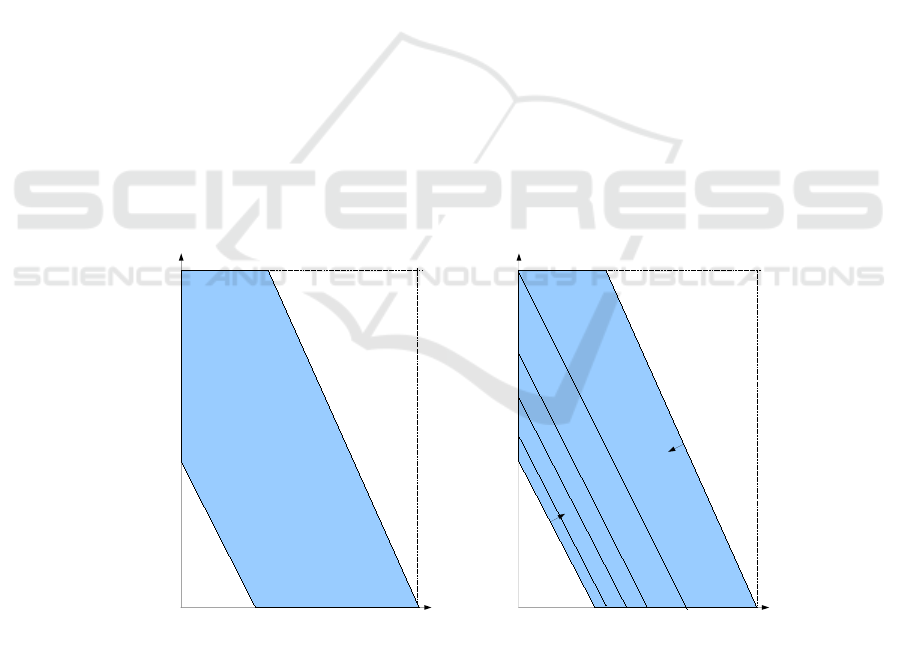
The actual polyhedron describing the solution space is depicted in Fig. 2.
X
Y
750
1000
214
428.5
0
X
Y
750
A=0.2
B=0.1
1000
428.5
0
214
A=0.7
B=0.35
250
A=0.6,
B=0.3
300
A=0.5
B=0.25
600
500
375
A=0.4,
B=0.2
750
500
A=0.3
B=0.15
Fig. 2. Left: Solution space. Tight and certain bounds for the decision variables: [0, 750] [0,
1000]. Right: Solution vectors of problem instances with consistent parameter solutions.
75
El MUNDO: Embedding Measurement Uncertainty in Decision Making and Optimization
75

We now give the intuition of our approach. The idea is to first solve the parameter
dependency constraints alone to obtain solution tuples, not intervals. To do so we use
a traditional branch and bound algorithm. We obtain a set of tuples for A and B such
that for each tuple the constraint A = 2 ∗ B holds. The idea is to have a well distributed
sample of solutions for this parameter constraint.
We obtain a set of tuples that satisfy the parameter constraint, in this case for in-
stance (0.2, 0.1), (0.3, 0.15), (0.4, 0.2), (0.5, 0.25), (0.6, 0.3), (0.7, 0.35). We then sub-
stitute each tuple in the uncertain constraint model rendering it a standard constraint
problem, and solve each instance. We record the solution matching each tuple instance.
The issue now is that even though we have a set of solutions for each tuple of param-
eters, there is no indication how the solutions evolve with the data. The tuples might
only represent a small set within the uncertainty range. The idea is to apply a regression
analysis between both. The regression function obtained shows the potential relation-
ship between the data parameters, that do satisfy the parameter constraints, and the
solutions. In this small example we can visualize how the solution evolves with the
data, see Fig. 2 on the right. In the case of much larger data sets, a tool like Matlab can
be used to compute the regression function and display the outcome. The algorithm and
complexity analysis are given in the following section.
3.2 Methodology and Algorithm
Our methodology is a three-steps iterative process: 1) Extract the uncertain parame-
ter constraints from the uncertain optimization problem and run branch and bound to
produce a set of tuple solutions, 2) solve a sequence of standard constraint optimiza-
tion problems where the tuples are being substituted to the uncertain parameters. This
is a simulation process that produces, if it exists, one solution per tuple instance. And
finally, 3) run a regression analysis on the parameter instances and their respective so-
lution, to identify the relationship function showing how the solutions evolve relative to
the with consistent parameters. The overall algorithmic process is given in Fig. 3. The
outcome of each step is highlighted in italic bold.
A constraint satisfaction and optimization problem, or CSOP, is a constraint satis-
faction problem (CSP) that seeks complete and consistent instantiations optimizing a
cost function. We use the notion of uncertain CSOP, or UCSOP first introduced in [23].
It extends a classical CSOP with uncertain parameters.
Uncertain CSOP and Uncertain Parameter Constraints. We first recall a CSOP. It
is commonly specified as a tuple (X , D, C, f ), where
– X is a finite set of variables,
– D is the set of corresponding domains,
– C = {c
1
, . . . , c
m
} is a finite set of constraints,
– f is the objective function over a a subset of the variables.
Definition 1 (UCSOP). An uncertain constraint satisfaction and optimization problem
is a classical CSOP in which some of the constraints may be uncertain, and is specified
by the tuple (X , D, C
X
, Λ, U, f). The finite set of parameters is denoted by Λ, and the
76
EPS Lisbon January 2015 2015 - European Project Space on Intelligent Systems, Pattern Recognition and Biomedical Systems
76

UCSOP
Constraint
simulation
Generator of
CSOP
instances
Parameter
constraints
Solution
Solution
set
set
Relationship function between
Relationship function between
uncertain data and solutions
uncertain data and solutions
Regression
analysis
Problem
constraints
Variables
Solution to each
Solution to each
CSOP
CSOP
Parameter
instances
Parameter
Parameter
tuples
tuples
Objective
function
Fig. 3. Process.
set of ranges for the parameters by U. A solution to a UCSOP is a solution space
enclosing safely the set of possible solutions.
Example 2. Let X
1
∈ D
1
and X
2
∈ D
2
both have domains D
1
= D
2
= [1.0..7.0].
Let λ
1
and λ
2
be parameters with uncertainty sets U
1
= [2.0..4.0] and U
2
= [1.0..6.0]
respectively. Consider three constraints:
C
1
: X
1
> λ
1
, C
2
: X
1
= X
2
+ λ
2
, C
3
: X
2
> 2
and the objective function to maximize f (X
1
, X
2
) = X
1
+ X
2
. This problem denotes
the UCSOP (X , D, C
X
, Λ, U, f) where X = {X
1
, X
2
}, D = {D
1
, D
2
}, Λ = {λ
1
, λ
2
},
U = {U
1
, U
2
}, and C
X
= {C
1
, C
2
, C
3
}.
Note that C
3
is a classical certain constraint; C
1
and C
2
are both uncertain con-
straints because they contain uncertain parameters. If now we add a constraint over the
paramaters such as C
4
: λ
2
= λ
1
+ 3, the set of parameter constraints is C
Λ
= {C
4
}.
Constraint Simulation. We now present our approach to solve a UCSOPs with pa-
rameter constraints, by transforming it into a set of tractable CSOPs instances where
the parameter constraints hold. More formally, we consider a UCSOP (X , D, C
X
∪
C
Λ
, Λ, U, f).
Definition 2 (Instance of UCSOP). Let us denote by n the number of variables, m the
number of uncertain parameters, p the number of parameter constraints, and inst(U
i
)
a value within the range of an uncertainty set. An instance of a UCSOP is a certain
CSOP (X , D, C
X
) such that for each uncertain constraint C
i
(X
1
..X
m
, λ
1
, ..λ
m
), we
have λ
j
= inst(U
j
), such that ∀k ∈ {1, .., p}, the parameter constraint C
k
(λ
1
, ..λ
m
)
is satisfied.
77
El MUNDO: Embedding Measurement Uncertainty in Decision Making and Optimization
77

Example 3. Continuing example 2, the UCSOP has two possible instances such that the
parameter constraint λ
2
= λ
1
+ 3 holds, given that λ
1
∈ U
1
, λ
2
∈ U
2
. The valid tuples
(λ
1
, λ
2
) are (2, 5), and (3, 6). The CSOP instances we generate are:
C
1
: X
1
> 2, C
2
: X
1
= X
2
+ 5, C
3
: X
2
> 2
and
C
1
: X
1
> 3, C
2
: X
1
= X
2
+ 6, C
3
: X
2
> 2
with the same objective function to maximize f = X
1
+ X
2
.
The generator of CSOP instances extracts the parameter constraints, polynomial in
the number of constraints in the worst case, then generates a set of parameter tuples
that satisfy these constraints. We can use a branch and bound search on the parameter
constraints of the UCSOP. The constraint simulation then substitutes the tuple solu-
tions onto the original UCSOP to search for a solution to each generated CSOP. This is
polynomial in the complexity of the UCSOP. The process is depicted in Algorithm 1.
Algorithm 1. Generate and solve CSOPs from one UCSOP.
Input: A UCSOP (X , D, C
X
∪ C
Λ
, Λ, U, f )
Output: Solutions to the CSOPs
1 SolsT uples ← ∅
2 extract(C
Λ
)
3 T uples ← solveBB(Λ, U, C
Λ
)
4 for T
i
∈ T uples do
5 substitute Λ with T
i
in (X , D, C
X
, Λ, f)
6 S
i
← solveOpt(X , D, C
X
, T
i
, f )
7 SolsT uples ← SolsT uples ∪ {(S
i
, T
i
)}
8 return SampleSols
Regression Analysis. The final stage of our process is to run a regression analy-
sis between the parameter solution tuples T ∈ T uples and the corresponding sol ∈
SolsT uples to estimate the relationship between the variations in the uncertain param-
eters called independent variables in regression analysis, and the solutions we com-
puted, called dependent variables. Using the common approach we can model a linear
regression analysis or one that minimizes the least-squares of errors.
Let us consider a linear regression, and the notation we used for the constraint
model, where T
i
is one parameter tuple, S
i
the associated solution produced. We as-
sume that the parameter instances were selected such that they are normally distributed
in the first place. There are d of them. The regression model takes the following form.
β is the regression coefficient to be found, and  the noise. The regression model is then
solved using MATLAB as a blackbox.
S = βT + 
where
S =




S
1
S
2
...
S
d




, T =




T
1
T
2
...
T
d




, β =




β
1
β
2
...
β
d




,  =





1

2
...

d




78
EPS Lisbon January 2015 2015 - European Project Space on Intelligent Systems, Pattern Recognition and Biomedical Systems
78

3.3 Illustration of the Methodology
We illustrate the benefits of our approach by solving an uncertain constraint optimiza-
tion problem, the traffic matrix estimation for the sigcomm4 problem, given in Fig. 1.
The topology and data values can be found in [16, 23]. Given traffic measurements over
each network link, and the traffic entering and leaving the network at the routers, we
search the actual flow routed between every pair of routers. To find out how much traffic
is exchanged between every pair of routers, we model the problem as an uncertain opti-
mization problem that seeks the min and max flow between routers such that the traffic
link and traffic conservation constraints hold. The traffic link constraints state that the
sum of traffic using the link is equal to the measured flow. The traffic conservation con-
straints, two per router, state that the traffic entering the network must equal the traffic
originating at the router, and the traffic leaving the router must equal the traffic whose
destination is the router.
We compare three models. The first one does not consider any uncertain parame-
ters and simplifies the model to only the variables in bold with coefficient 1. The traffic
between routers takes a single fixed path, as implemented in [16]. The second model
extends the first one with uncertain parameters but without the parameter dependency
constraints. The third one is our approach with the parameter dependency constraints
added. A parameter constraint, over the flow F
AB
, for instance, states that the coef-
ficients representing one given route of traffic from A to B take the same value; and
the sum of coefficients corresponding to different routes equals to 1. Note that the un-
certain parameter equality constraints are already taken into account in the link traffic
constraints. The uncertain parameters relative to flow distributions are commonly as-
sumed between 30 and 70 % [23]. The distribution of split traffic depends mainly on
the duration of traffic sampling, the configuration of the routers, and the routing proto-
col itself.
Decision variables:
[F
AB
, F
AC
, F
AD
, F
BA
, F
BC
, F
BD
, F
CA
, f
CB
, F
CD
, F
DA
, F
DB
, F
DC
] ∈ 0.0..100000
Parameters:
[λ
1
AB
, λ
1
AC
, λ
1
AD
, λ
1
BC
, λ
1
BD
, λ
2
AB
, λ
2
AC
, λ
2
AD
, λ
2
BC
, λ
2
BD
] ∈ 0.3..0.7
Link traffic constraints:
A → B λ
1
AB
∗ F
AB
+ λ
1
AC
∗ F
AC
+ λ
1
AD
∗ F
AD
= 309.0..327.82
B → A F
BA
+ F
CA
+ F
DA
+ λ
1
BC
∗ F
BC
+ λ
1
BD
∗ F
BD
= 876.39..894.35
A → C λ
2
AC
∗ F
AC
+ λ
2
AD
∗ F
AD
+ λ
2
AB
∗ F
AB
+ λ
1
BC
∗ F
BC
+
λ
1
BD
∗ F
BD
= 591.93..612.34
B → C λ
2
BC
∗ F
BC
+ λ
2
BD
∗ F
BD
+ λ
1
AC
∗ F
AC
+ λ
1
AD
∗ F
AD
= 543.30..562.61
C → B λ
2
AB
∗ F
AB
+ F
CB
+ F
CA
+ F
DA
+ F
DB
= 1143.27..1161
C → D F
CD
+ F
BD
+ F
AD
= 896.11..913.98
D → C F
DC
+ F
DB
+ F
DA
= 842.09..861.35
Parameter constraints
λ
1
AB
+ λ
2
AB
= 1, λ
1
AC
+ λ
2
AC
= 1, λ
1
AD
+ λ
2
AD
= 1, λ
1
BC
+ λ
2
BC
= 1
79
El MUNDO: Embedding Measurement Uncertainty in Decision Making and Optimization
79

Traffic conservation constraints
A origin F
AD
+ F
AC
+ F
AB
= 912.72..929.02
A destination F
DA
+ F
CA
+ F
BA
= 874.70..891.00
B origin F
BD
+ F
BC
+ F
BA
= 845.56..861.86
B destination F
DB
+ F
CB
+ F
AB
= 884.49..900.79
C origin F
CD
+ F
CB
+ F
CA
= 908.28..924.58
C destination F
DC
+ F
BC
+ F
AC
= 862.53..878.83
D origin F
DC
+ F
DB
+ F
DA
= 842.0..859.0
D destination F
CD
+ F
BD
+ F
AD
= 891.0..908.0
Results. We first ran the initial model (constraints with variables in bold for the link
traffic together with the traffic conservation constraints) and reproduced the model and
results of [23]. We used the linear EPLEX solver. By adding the uncertain parameters
there was no solution at all. This indicates that not all traffic could be rerouted given the
traffic volume data given.
We then disabled the uncertainty over the traffic BD, maintaining its route through
the router C only. A solution set was found, with solution bounds much larger than the
initial bounds (without uncertain distribution). Indeed,the space of potential solutions
expanded. However, when we run simulations using our approach on the model with de-
pendency constraints, there was no solution to the model. This shows the importance of
taking into account such dependencies, and also indicates in this case the data provided
are very likely matching a single path routing algorithm for the sigcomm4 topology.
After enlarging the interval bounds of the input data we were able to find a solution
with a 50 % split of traffic, but none with 40 − 60 or other combinations. This exper-
imental study showed the strong impact of taking into account dependency constraints
with simulations [13].
Exploiting the Problem Structure. After completing this study, and running the simula-
tions, we identified that when the uncertain parameters are coefficients to the decision
variables and follow a certain problem structure, we can improve the efficiency of the
approach. Basically it became clear that the fact that the constraints on the uncertain
parameters tell us about the potential values of the decision variables and not whether
the problem is satisfiable or not. For instance, when we allow the traffic F
BD
to be
split, there was no solution. Possible interpretations are: 1) this distribution (30 − 70%)
is not viable and the problem is not solvable, 2) that there is no traffic between B and
D. In the latter case, the handling of the dependency constraints should be done hand in
hand with the labeling of the decision variables. This has been the subject of our second
approach [14].
4 Matrix Models
The main novel idea behind this approach is based on the study of the problem struc-
ture. We identify the context of matrix models where uncertain data correspond to co-
efficients of the decision variables, and the constraints over these apply to the columns
of the input matrix. Such data constraints state restrictions on the possible usage of the
80
EPS Lisbon January 2015 2015 - European Project Space on Intelligent Systems, Pattern Recognition and Biomedical Systems
80

data, and we show how their satisfaction can be handled efficiently in relationship with
the corresponding decision variables.
In this context, the role and handling of uncertain data constraints is to determine
”which data can be used, to build a solution to the problem”. This is in contrast with
standard constraints over decision variables, which role is to determine ”what value
can a variable take to derive a solution that holds”. We illustrate the context and our
new notion of uncertain data constraint satisfaction on a production planning problem
inspired from [15].
Example 4. Three types of products are manufactured, P
1
, P
2
, P
3
on two different ma-
chines M
1
, M
2
. The production rate of each product per machine is imprecise and spec-
ified by intervals. Each machine is available 9 hrs per day, and an expected demand per
day is specified by experts as intervals. Furthermore we know that the total production
rate of each machine cannot exceed 7 pieces per hour. We are looking for the number of
hours per machine for each product, to satisfy the expected demand. An instance data
model is given below.
Product Machine M1 Machine M2 Expected demand
P
1
[2, 3] [5, 7] [28, 32]
P
2
[2, 3] [1, 3] [25, 30]
P
3
[4, 6] [2, 3] [31, 37]
The uncertain CSP model is specified as follows:
[2, 3] ∗ X
11
+ [5, 7] ∗ X
12
= [28, 32] (1)
[2, 3] ∗ X
21
+ [1, 3] ∗ X
22
= [25, 30] (2)
[4, 6] ∗ X
31
+ [2, 3] ∗ X
32
= [31, 37] (3)
∀j ∈ {1, 2} : X
1j
+ X
2j
+ X
3j
≤ 9 (4)
∀i ∈ {1, 2, 3}, ∀j ∈ {1, 2} : X
ij
≥ 0 (5)
Uncertain data constraints:
a
11
∈ [2, 3], a
21
∈ [2, 3], a
31
∈ [4, 6], a
11
+ a
21
+ a
31
≤ 7 (6)
a
12
∈ [5, 7], a
22
∈ [1, 3], a
32
∈ [2, 3], a
12
+ a
22
+ a
32
≤ 7 (7)
Consider a state of the uncertain CSP such that X
11
= 0. The production rate of
machine M
1
for product P
1
becomes irrelevant since X
11
= 0 means that machine M
1
does not produce P
1
at all in this solution. The maximum production rate of M
1
does
not change but now applies to P
2
and P
3
. Thus X
11
= 0 infers a
11
= 0. Constraint (6)
becomes:
a
21
∈ [2, 3], a
31
∈ [4, 6], a
21
+ a
31
≤ 7 (8)
Assume now that we have a different production rate for P
3
on M
1
:
a
11
∈ [2, 3], a
21
∈ [2, 3], a
31
∈ [8, 10], a
11
+ a
21
+ a
31
≤ 7 (9)
P
3
cannot be produced by M
1
since a
31
∈ [8, 10]  7, the total production rate of M
1
is too little. This does not imply that the problem is unsatisfiable, but that P
3
cannot be
produced by M
1
. Thus a
31
 7 yields X
31
= 0 and a
31
= 0. 
81
El MUNDO: Embedding Measurement Uncertainty in Decision Making and Optimization
81

In this example we illustrated our interpretation of uncertain data dependency con-
straints, and how the meaning, role and handling of such constraints differs from stan-
dard constraints over decision variables. It must be different, and strongly tied with
the decision variables the data relates to, as these are the ones being pruned and in-
stantiated. In this following we formalize our approach by introducing a new notion of
relative consistency for dependency constraints, together with a model that offers an
efficient means to check and infer such consistency.
4.1 Formalization
We now formalize the context of matrix models we identified and the handling of un-
certain data constraints within it.
Problem Definition
Definition 3 (Interval Data). An interval data, is an uncertain data, specified by an
interval [a, a], where a (lower bound) and a (upper bound) are positive real numbers,
such that a ≤ a.
Definition 4 (Matrix Model with Column Constraints). A matrix model with uncer-
tain data constraints is a constraint problem or a component of a larger constraint
problem that consists of:
1. A matrix (A
ij
) of input data, such that each row i denotes a given product P
i
, each
column j denotes the source of production and each cell a
ij
the quantity of product
i manufactured by the source j. If the input is bounded, we have an interval input
matrix, where each cell is specified by [a
ij
, a
ij
].
2. A set of decision variables X
ij
∈ R
+
denoting how many instances of the corre-
sponding input shall be manufactured
3. A set of column constraints, such that for each column j: Σ
i
[a
ij
, a
ij
] @ c
j
, where
@ ∈ {=, ≤}, and c
j
can be a crisp value or a bounded interval.
The notion of (interval) input matrix is not to be confused with the Interval Lin-
ear Programming matrix (ILP) model in the sense that an ILP matrix is driven by the
decision vector and the whole set of constraints as illustrated in the example below.
Example 5. The interval input matrix for the problem in example 2 is:


[a
11
, a
11
] [a
12
, a
12
]
[a
21
, a
21
] [a
22
, a
22
]
[a
31
, a
31
] [a
32
, a
32
]


=


[2, 3] [5, 7]
[2, 3] [1, 3]
[4, 6] [2, 3]


The ILP matrix for this problem is:






[2,3] [5,7] 0 0 0 0
0 0 [2,3] [1,3] 0 0
0 0 0 0 [4,6] [2,3]
1 0 1 0 1 0
0 1 0 1 0 1






82
EPS Lisbon January 2015 2015 - European Project Space on Intelligent Systems, Pattern Recognition and Biomedical Systems
82

The decision vector for the ILP matrix is [X
11
, X
12
, X
21
, X
22
, X
31
, X
32
].
To reason about uncertain matrix models we make use of the robust counterpart
transformation of interval linear models into linear ones. We recall it, and define the
notion of relative consistency of column constraints.
Linear Transformation. An Interval Linear Program is a Linear constraint model
where the coefficients are bounded real intervals [9, 3]. The handling of such models
transforms each interval linear constraint into an equivalent set of atmost two standard
linear constraints. Equivalence means that both models denote the same solution space.
We recall the transformations of an ILP into its equivalent LP counterpart.
Property 1 (Interval linear constraint and equivalence). Let all decision variables X
il
∈
R
+
, and all interval coefficients be positive as well. The interval linear constraint C =
Σ
i
[a
il
, a
il
] ∗ X
il
@ [c
l
, c
l
] with @ ∈ {≤, =}, is equivalent to the following set of
constraints depending on the nature of @. We have:
1. C = Σ
i
[a
il
, a
il
] ∗ X
il
≤ [c
l
, c
l
] is transformed into: C = Σ
i
a
il
∗ X
il
≤ c
l
2. C = Σ
i
[a
il
, a
il
] ∗ X
il
= [c
l
, c
l
] is transformed into:
C = {Σ
i
a
il
× X
il
≤ c
l
∧ Σ
i
a
il
∗ X
il
≥ c
l
}
Note that case 1 can take a different form depending on the decision maker risk
adversity. If he assumes the highest production rate for the smallest demand (pessimistic
case), the transformation would be: C = Σ
i
a
il
∗X
il
≤ c
l
. The solution set of the robust
counterpart contains that of the pessimistic model.
Example 6. Consider the following constraint a
1
∗ X + a
2
∗ Y = 150 (case 2), with
a
1
∈ [0.2, 0.7], a
2
∈ [0.1, 0.35], X, Y ∈ [0, 1000]. It is rewritten into the system of
constraints: l
1
: 0.7 ∗ X + 0.35 ∗ Y ≥ 150 ∧ l
2
: 0.2 ∗ X + 0.1 ∗ Y ≤ 150.
X
Y
750
1000
214
428.5
0
X
Y
750
a1=0.2
a2=0.1
1000
428.5
0
214
a1=0.7
a2=0.35
250
,
600
500
750
l2
l2
l1
l1
Fig. 4. Left: Solution space. Reliable bounds for the decision variables: [0, 750] [0, 1000]. Right:
Solution space bounded by the constraints l
1
and l
2
.
83
El MUNDO: Embedding Measurement Uncertainty in Decision Making and Optimization
83

The polyhedron describing the solution space (feasible region) for X and Y is de-
picted in Fig. 4 (left), together with the boundary lines l
1
and l
2
, representing the two
constraints above.
The transformation procedure also applies to the column constraints, and is denoted
transf. It evaluates to true or false since there is no variable involved.
Relative Consistency. We now define in our context, the relative consistency of column
constraints with respect to the decision variables. At the unary level this means that if
(X
ij
= 0) then (a
ij
= 0), if ¬ transf(a
ij
@c
j
) then (X
ij
= 0) and if X
ij
> 0 then
transf(a
ij
@ c
j
) is true.
Definition 5 (Relative Consistency). A column constraint Σ
i
a
il
@ c
l
over the column
l of a matrix I ∗ J , is relative consistent w.r.t. the decision variables X
il
if and only if
the following conditions hold (C4. and C5. being recursive):
C1. ∀i ∈ I such that X
il
> 0, we have transf(Σ
i
a
il
@ c
l
) is true
C2. ∀k ∈ I such that {¬transf(Σ
i6=k
a
il
@ c
l
) and transf(Σ
i
a
il
@ c
l
)} is true, we
have X
kl
> 0
C3. ∀i ∈ I such that X
il
is free, transf(Σ
i
a
il
@ c
l
) is true
C4. ∀k ∈ I, such that ¬transf(a
kl
@ c
l
), we have X
kl
= 0 and Σ
i6=k
a
il
@ c
l
is
relative consistent
C5. ∀k ∈ I, such that X
kl
= 0, we have Σ
i6=k
a
il
@ c
l
is relative consistent
Example 7. Consider the Example 1. It illustrates cases C4. and C5, leading to a recur-
sive call to C3. Let us assume now that the X
i1
are free, and that we have the column
constraint [2, 3] + [2, 3] + [4, 6] = [7, 9]. Rewritten into 2 + 2 + 4 ≤ 9, 3 + 3 + 6 ≥ 7,
we have X
31
> 0, since 3 + 3 6≥ 7 and 3 + 3 + 6 ≥ 7. It is relative consistent with
X
31
> 0 (C2.).
Similarly if we had an uncertain data constraint limiting the total production rate of
M
1
to 5 and a
31
∈ [6, 7], yielding the column constraint:
a
11
∈ [2, 3], a
21
∈ [2, 3], a
31
∈ [6, 7], a
11
+ a
21
+ a
31
≤ 5
With all X
i1
free variables this column constraint is not relative consistent, since the
transformed relation is 2 + 2 + 6 ≤ 5. P
3
cannot be produced by M
1
because the
maximum production rate of M
1
is too little (6  5, and condition 3 fails). This does
not mean that the problem is unsatisfiable! Instead, the constraint can become relative
consistent by inferring X
31
= 0 and a
31
= 0, since the remainder a
11
+ a
21
≤ 5 is
relative consistent (condition 3 holds). M
1
can indeed produce P
1
and P
2
. 
4.2 Column Constraint Model
Our intent is to model column constraints and infer relative consistency while preserv-
ing the computational tractability of the model. We do so by proposing a Mixed Integer
Interval model of a column constraint. We show how it allows us to check and infer rel-
ative consistency efficiently. This model can be embedded in a larger constraint model.
The consistency of the whole constraint system is inferred from the local and relative
consistency of each constraint.
84
EPS Lisbon January 2015 2015 - European Project Space on Intelligent Systems, Pattern Recognition and Biomedical Systems
84

Modeling Column Constraints. Consider the column constraint over column l :
Σ
i
[a
il
, a
il
] @ c
l
.
It needs to be linked with the decision variables X
il
. Logical implications could be
used, but they would not make an active use of consistency and propagation techniques.
We propose an alternative MIP model.
First we recall the notion of bounds consistency we exploit here.
Definition 6 (Bound Consistency). [1] An n-ary constraint is Bound Consistent (BC),
iff for each bound of each variable there exists a value in each other variable’s domain,
such that the constraint holds.
A constraint system with column constraints is BC if each constraint is BC.
Example 8. The constraint X ∈ [1, 2], Y ∈ [2, 4], Z ∈ [1, 2], X + Y + Z = 5 is not
bounds consistent because the value Y = 4 cannot participate in a solution. Once the
domain of Y is pruned to [2, 3], the constraint is BC.
New Model. To each data we associate a Boolean variable. Each indicates whether:
1) the data must be accounted for to render the column constraint consistent, 2) the
data violates the column constraint and needs to be discarded, 3) the decision variable
imposes a selection or removal of the data. Thus the column constraint in transformed
state is specified as a scalar product of the data and Boolean variables. The link between
the decision variables and their corresponding Booleans is specified using a standard
mathematical programming technique that introduces a big enough positive constant
K, and a small enough constant λ.
Theorem 1 (Column Constraint Model). Let X
il
∈ R
+
be decision variables of the
matrix model for column l. Let B
il
be Boolean variables. Let K be a large positive
number, and λ a small enough positive number. A column constraint
Σ
i
[a
il
, a
il
] @ c
l
is relative consistent if the following system of constraints is bounds consistent
transf(Σ
i
[a
il
, a
il
] × B
il
@ c
l
) (10)
∀i, 0 ≤ X
il
≤ K × B
il
(11)
∀i, λ × B
il
≤ X
il
(12)
Proof. The proof assumes that the system of constraints (10-12) is BC and proves that
this entails that the column constraint is relative consistent. Note that constraint (10) is
transformed into an equivalent linear model using the transformation procedure given
in Section 4.1 relative to the instance of @ used.
If the system of constraints is BC, by definition each constraint is BC. If all X
il
are
free, so are the B
il
(they do not appear elsewhere), and since (10) is BC then condition
3 holds and the column constraint is relative consistent. If some of the X
il
are strictly
positive and ground, the corresponding Booleans are set to 1 (since 11 is BC), and given
that (10) is BC by supposition, condition 3 holds and the column constraint is relative
consistent. If some of the X
il
are ground to 0, so are the corresponding B
il
since (12) is
BC, and since (10) is BC, condition 3 holds (the remaining decision variables are either
strictly positive or free and constraint (10) is BC).
85
El MUNDO: Embedding Measurement Uncertainty in Decision Making and Optimization
85

Complexity. For a given column constraint, if we have n uncertain data (thus n related
decision variables), our model generates n Boolean variables and O(2n + 2) = O(n)
constraints. This number is only relative to the size of a column and does not depend on
the size or bounds of the uncertain data domain.
4.3 Column Constraints in Optimization Models
The notion of Bounds Consistency for a constraint system ensures that all possible
solutions are kept within the boundaries that hold. As we saw, for the column constraints
this means that resources that can’t be used (do not satisfy the dependency) cannot be
selected to contribute to the solutions, and those that must be used are included in the
potential solution.
Such an approach is not limited to decision problems, it can be easily embedded in
optimization models. An optimization problem with bounded data can be solved using
several objective functions such as minmax regret or different notions of robustness.
Our column constraint model can naturally be embedded in any uncertain optimization
problems provided an input matrix model is associated with the specification of the
uncertain data dependency constraints. Side constraints can be of any form.
The only element to be careful about is the transformation model chosen for the
column constraints. The one given in Section 4.1. is the robust one that encloses all
possible solutions. However, depending on the risk adversity of the decision maker
some more restrictive transformations can be used as we discussed. Clearly if the whole
problem can be modelled as a Mixed Integer Problem (MIP), MIP solvers can be used.
4.4 Illustration of the Matrix Model Approach
We illustrate the approach on the production planning problem. The robust model is
specified below. Each interval linear core constraint is transformed into a system of two
linear constraints, and each column constraint into its robust counterpart.
For the core constraints we have:
2 ∗ X
11
+ 5 ∗ X
12
≤ 32, 3 ∗ X
11
+ 7 ∗ X
12
≥ 28,
2 ∗ X
21
+ X
22
≤ 30, 3 ∗ X
21
+ 3 ∗ X
22
≥ 25,
4 ∗ X
31
+ 2 ∗ X
32
≤ 37, 6 ∗ X
31
+ 3 ∗ X
32
≥ 31,
∀j ∈ {1, 2}, X
1j
+ X
2j
+ X
3j
≤ 9,
∀i ∈ {1, 2, 3}, ∀j ∈ {1, 2} : X
ij
≥ 0,
∀i, j, X
ij
≥ 0, B
ij
∈ {0, 1},
86
EPS Lisbon January 2015 2015 - European Project Space on Intelligent Systems, Pattern Recognition and Biomedical Systems
86

And for the column constraints:
a
11
∈ [2, 3], a
21
∈ [2, 3], a
31
∈ [4, 6], a
11
+ a
21
+ a
31
≤ 7 and
a
12
∈ [5, 7], a
22
∈ [1, 3], a
32
∈ [2, 3], a
12
+ a
22
+ a
32
≤ 7 transformed into:
2 ∗ B
11
+ 2 ∗ B
21
+ 4 ∗ B
31
≤ 7,
5 ∗ B
12
+ B
22
+ 2 ∗ B
32
≤ 7,
∀i ∈ {1, 2, 3}, j ∈ {1, 2} 0 ≤ X
ij
≤ K ∗ B
ij
,
∀i ∈ {1, 2, 3}, j ∈ {1, 2} λ ∗ B
ij
≤ X
ij
We consider three different models: 1) the robust approach that seeks the largest
solution set, 2) the pessimistic approach, and 3) the model without column data con-
straints. They were implemented using the ECLiPSe ic interval solver [8]. We used
the constants K=100 and λ = 1. The column constraints in the tightest model take the
form: 3 ∗ B
11
+ 3 ∗ B
21
+ 6 ∗ B
31
≤ 7 and 7 ∗ B
12
+ 3 ∗ B
22
+ 3 ∗ B
32
≤ 7.
The solution set results are summarized in the following table with real values
rounded up to hundredth for clarity. The tightest model, where the decision maker as-
sumes the highest production rates has no solution.
Variables With column constraints Without column constraints
Robust model Tightest model
Booleans Solution bounds Solution bounds Solution bounds
X
11
0 0.0..0.0 − 0.0 .. 7.00
X
12
1 4.0..4.5 − 0.99 .. 6.4
X
21
1 3.33..3.84 − 0.33 .. 7.34
X
22
1 4.49..5.0 − 0.99 .. 8.0
X
31
1 5.16..5.67 − 1.66 ..8.67
X
32
0 0.0..0.0 − 0.0 .. 7.0
Results. From the table of results we can clearly see that:
1. Enforcing Bounds Consistency (BC) on the constraint system without the column
constraints, is safe since the bounds obtained enclose the ones of the robust model
with column constraints. However, they are large, and the impact of accounting for
the column constraints, both in the much reduced bounds obtained, and to detect
infeasibility is shown.
2. The difference between the column and non column constraint models is also in-
teresting. The solutions show that only X
11
and X
32
can possibly take a zero value
from enforcing BC on the model without column constraints. Thus all the other
decision variables require the usage of the input data resources. Once the column
constraints are enforced, the input data a
11
and a
32
must be discarded since oth-
erwise the column constraints would fail. This illustrates the benefits of relative
consistency over column constraints.
3. The tightest model fails, because we can see from the solution without column
constraints that a
21
and a
31
must be used since their respective X
ij
are strictly
positive in the solution to the model without column constraints. However from the
87
El MUNDO: Embedding Measurement Uncertainty in Decision Making and Optimization
87

tight column constraint they can not both be used at full production rate at the same
time. The same holds for a
12
and a
22
.
All computations were performed in constant time given the size of the problem.
This approach can easily scale up, since if we have n uncertain data (thus n related
decision variables) in the matrix model, our model generates n Boolean variables and
O(2n + 2) = O(n) constraints. This number does not depend on the size or bounds
of the uncertain data domain, and the whole problem models a standard CP or MIP
problem, making powerful use of existing techniques.
5 Conclusion
In this paper we introduced two multi-disciplinary approaches to account for depen-
dency constraints among data parameters in an uncertain constraint problem. The first
approach follows an iterative process that first satisfies the dependency constraints using
a branch and bound search. The solutions are then embedded to generate a set of CSPs
to be solved. However this does not indicate the relationship between the dependent
consistent parameters and possible solutions. We proposed to use regression analysis
to do so. The current case study showed that by embedding constraint dependencies
only one instance had a solution. This was valuable information on its own, but limited
the use of regression analysis. Further experimental studies are underway with appli-
cations in inventory management, problems clearly permeated with data uncertainty.
This directed us towards the second approach where we identified a the structure of
matrix models to account for uncertain data constraints in relationship with the deci-
sion variables. Such models are common in many applications ranging from production
planning, economics, inventory management, or network design to name a few. We de-
fined the notion of relative consistency, and a model of such dependency constraints that
implements this notion effectively. The model can be tackled using constraint solvers
or MIP techniques depending on the remaining core constraints of the problem. Further
experimental studies are underway with applications to large inventory management
problems clearly permeated with such forms of data uncertainty and dependency con-
straints. An interesting challenge to our eyes, would be to investigate how the notion
of relative consistency can be generalized and applied to certain classes of global con-
straints in a CP environment, whereby the uncertain data appears as coefficients to the
decision variables. Even though our approaches have been applied to traditional con-
straint problems in mind, their benefits could be stronger on data mining applications
with constraints [10].
References
1. Benhamou, F. Inteval constraint logic programming. In Constraint Programming: Basics
and Trends. LNCS, Vol. 910, 1-21, Springer, 1995.
2. Benhamou F. and Goualard F. Universally quantified interval constraints. In Proc. of CP-
2000, LNCS 1894, Singapore, 2000.
3. Ben-Tal, A; and Nemirovski, A. Robust solutions of uncertain liner programs. Operations
Research Letters, 25, 1-13, 1999.
88
EPS Lisbon January 2015 2015 - European Project Space on Intelligent Systems, Pattern Recognition and Biomedical Systems
88

4. Bertsimas, D. and Brown, D. Constructing uncertainty sets for robust linear optimization.
Operations Research, 2009.
5. Bordeaux L., and Monfroy, E. Beyond NP: Arc-consistency for quantified constraints. In
Proc. of CP 2002.
6. Boukezzoula R., Galichet S. and Bisserier A. A MidpointRadius approach to regression with
interval data International Journal of Approximate Reasoning,Volume 52, Issue 9, 2011.
7. Brown K. and Miguel I. Chapter 21: Uncertainty and Change Handbook of Constraint
Programming Elsevier, 2006.
8. Cheadle A.M., Harvey W., Sadler A.J., Schimpf J., Shen K. and Wallace M.G. ECLiPSe: An
Introduction. Tech. Rep. IC-Parc-03-1, Imperial College London, London, UK.
9. Chinneck J.W. and Ramadan K. Linear programming with interval coefficients. J. Opera-
tional Research Society, 51(2):209–220, 2000.
10. De Raedt L., Mannila H., O’Sullivan and Van Hentenryck P. organizers. Constraint Program-
ming meets Machine Learning and Data Mining Dagstuhl seminar 2011.
11. Fargier H., Lang J. and Schiex T. Mixed constraint satisfaction: A framework for decision
problems under incomplete knowledge. In Proc. of AAAI-96, 1996.
12. Gent, I., and Nightingale, P., and Stergiou, K. QCSP-Solve: A Solver for Quantified Con-
straint Satisfaction Problems. In Proc. of IJCAI 2005.
13. Gervet C. and Galichet S. On combining regression analysis and constraint programming.
Proceedings of IPMU, 2014.
14. Gervet C. and Galichet S. Uncertain Data Dependency Constraints in Matrix Models. Pro-
ceedings of CPAIOR, 2015.
15. Inuiguchi, M. and Kume, Y. Goal programming problems with interval coefficients and
target intervals. European Journl of Oper. Res. 52, 1991.
16. Medina A., Taft N., Salamatian K., Bhattacharyya S. and Diot C. Traffic Matrix Estimation:
Existing Techniques and New Directions. Proceedings of ACM SIGCOMM02, 2002.
17. Oettli W. On the solution set of a linear system with inaccurate coefficients. J. SIAM: Series
B, Numerical Analysis, 2, 1, 115-118, 1965.
18. Ratschan, S. Efficient solving of quantified inequality constraints over the real numbers.
ACM Trans. Computat. Logic, 7, 4, 723-748, 2006.
19. Rossi F., van Beek P., and Walsh T. Handbook of Constraint Programming. Elsevier, 2006.
20. Saad A., Gervet C. and Abdennadher S. Constraint Reasoning with Uncertain Data
usingCDF-Intervals Proceedings of CP’AI-OR, Springer,2010.
21. Van Hentenryck P., Michel L. and Deville Y. Numerica: a Modeling Language for Global
Optimization The MIT Press, Cambridge Mass, 1997.
22. Tarim, S. and Kingsman, B. The stochastic dynamic production/inventory lot-sizing prob-
lem with service-level constraints. International Journal of Production Economics 88,
105119,2004.
23. Yorke-Smith N. and Gervet C. Certainty Closure: Reliable Constraint Reasoning with Un-
certain Data ACM Transactions on Computational Logic 10(1), 2009.
89
El MUNDO: Embedding Measurement Uncertainty in Decision Making and Optimization
89