Fast Direction-of-Arrival Estimation for Single Source
Near- and Far-Field Approaches for 1D Source Localization
Iurii Chyrka
Institute of Information and Communication Technologies, Bulgarian Academy of Sciences,
25A, Acad. G. Bonchev str., 1113 Sofia, Bulgaria
Keywords: Direction-of-Arrival Estimation, Far-field, Near-field, Source Localization, Autoregressive Moving
Average Model, Spatial Frequency Estimation.
Abstract: The new approaches for a single narrowband source direction-of-arrival estimation in a far-field scenario
and both direction-of-arrival and range estimation a near-field scenario are proposed. The main idea is to
estimate the spatial frequency directly along the uniform linear array aperture from the single-shot
measurement. The algorithm based on the autoregressive moving average model of the sinewave is applied
for the frequency estimation. The effectiveness of proposed methods is analysed via computer simulations.
1 INTRODUCTION
The problem of direction-of-arrival (DOA)
estimation of multiple plane waves generated by
narrowband signal sources have attracted
considerable interest in the literature due to a variety
of applications in communication, seismology,
oceanography, radar, acoustics, and so on. This
problem is considered in the framework of the array
signal processing and signal parameter estimation in
particular. Usually the objective is to estimate
parameters, such as azimuth, elevation, range, center
frequency etc. associated with each signal.
Localization problem can be generally divided
into two types, based on the distance between the
source and the antenna array: far-field (when
 /2
2
Dr
, r is the range between the source and
the array reference point, D is the array aperture, λ is
the wavelength of the source signal), and near-field
localization. In far-field case, the wavefront of the
signal impinging on the array is assumed to be
planar (Johnson, 2006). When the source is located
in the Fresnel region (
 /2/62.0
23
DrD
) or
even closer in the near-field
 /62.0
3
Dr
the
wave front gets some curvature. It is reasonable to
split processing algorithms onto ones based on the
planar wave assumption and ones for the circular
wavefront.
For the far-field estimation there are a lot of
methods that can be separated onto three categories.
The first one is beamforming algorithms like delay-
and-sum or minimum variance distortionless
response (Bai, Ih, Benesty, 2013), which obtain a
nonparametric spatial spectrum by application of a
data-adaptive spatial filtering. The subspace
algorithms like MUSIC (Stoica, Nehorai, 1989),
ESPRIT (Gao, Gershman 2005) use the low-rank
structure of the noise-free signal. The maximum
likelihood methods (Wax, 1982), (Stoica, Besson,
2000), (Chen, Lorenzelli, Hudson, Yao, 2008) work
with statistical properties, but require precise
initialization to ensure convergence to a global
minimum. Due statistical nature, they need
sufficiently big data amount for accurate estimation.
In the case of single source localization, direction
finding of the narrowband singal can be interpreted
as a problem of a sinewave signal parameter
estimation, particularly estimation of the spatial
frequency. Besides, reduction of the problem allows
using of simplified algorithms. (Wu, Liu, So, 2009).
In the near-field scenario it is necessary to
estimate simultaneously two position parameters: a
pair of coordinates or DOA and range. Therefore,
traditional approaches like MUSIC must be
extended to a two-dimensional field. Swindlehurst
and Kailath (1988) suggest a quadratic (Fresnel)
approximation of the wavefront in the near-field.
54
Chyrka I.
Fast Direction-of-Arrival Estimation for Single Source - Near- and Far-Field Approaches for 1D Source Localization.
DOI: 10.5220/0005889400540058
In Proceedings of the Fourth International Conference on Telecommunications and Remote Sensing (ICTRS 2015), pages 54-58
ISBN: 978-989-758-152-6
Copyright
c
 2015 by SCITEPRESS – Science and Technology Publications, Lda. All rights reserved

Using this approximation, the rotational invariance
property can be used with the symmetric subarrays
to estimate the DOA by ESPRIT (Zhi, Chia, 2007).
In the paper of (Grosocki, Abed-Meraim, Hua 2005)
position is obtained through estimation of two angles
by weighted linear prediction. Another approach of
transformation near-field localization problem to far-
field one via interpolation is considered in (Yang,
Shi, Liu, 2009).
In this work, we focus on the problem of
estimation the DOA of a single source in both far-
and near-field situations and the alternative approach
of single-shot direct estimation of the spatial
frequency from the one source is considered.
2 DOA ESTIMATION
ALGORITHMS
2.1 Far-field Scenario
Let us consider a single narrowband signal s(t) that
comes from far-field and its source is located far
enough to assume a wavefront as a linear one. The
signal is received from direction

by a uniform
linear array (ULA) of M sensors. In order to avoid
spatial aliasing distance d between them must be
lesser than a signal wavelength
c

.
The narrowband signal can be simply written as
the next time-harmonic dependence
)exp()()( ttAts
c

,
(1)
where A(t) is the baseband signal,
c

is the signal
center angular frequency.
The signal from far-field received by the
microphone array can be written as the next vector
).()()(
)(
)(
)(
),(
),(
),(
1
/)sin()1(2
/)sin(02
1
tts
t
t
ts
e
e
tx
tx
t
c
cM
c
Mdj
dj
M
ηα
x










































(2)
),( tx
m
is a signal captured by mth sensor,
)(t
c
η
is a
corresponding complex additive noise assumed as a
white Gaussian noise with zero mean,
)(α
is an
array manifold vector or the steering vector (Bai, et
al., 2013) that depends on the DOA

. One can see
that captured signals
)(tx
m
have constant phase shift
between each other
)sin( kd
,
c
k  /2
. This
shift is a spatial frequency that has to be estimated.
In many real situations the received signal is not
complex or sensors record only a real part of it. If
we assume that the received signal is a single-tone
one with an angular frequency
c

, amplitude A and
is sampled onto N samples with sampling interval

than in any discrete moment of time
)1(  nt
n
,
Nn ,1
can be described as
.
)(
)(
))1(sin(
)0sin(
),(
1


























nM
n
nc
nc
n
t
t
MtA
tA
t x
(3)
where
)(
nm
t
are real parts of the noise vector
)(t
c
η
in the equation.
The minimal sufficient information for frequency
estimation is contained in only the one vector
)(
n
tx
taken in any arbitrary moment of the discrete time.
Hence, for simplicity we can chose the n=1 and
write the corresponding measurement vector
m
mA  ))1(sin()(x
,
Mm ,1
.
(4)
For estimation of the spatial frequency in the
signal (4) the algorithm considered in the paper of
Prokopenko, Omelchuk, Chyrka (2012) is used. It is
based on the representation of the noised sinewave
signal as an autoregressive moving average model of
the second order. The DOA estimation procedure
with frequency estimation steps can be summarized
as follows:
a) calculation of the signal statistics
       














1
2
1mmm1m
1
2
2
m
2
1m1m
2/2
M
m
M
m
xxxxxxxxB
b) obtaining of two values of the autoregressive
model parameter
   
2
ˆ
2
)2(1
 xBxB
;
c) spatial frequency estimation
 
2/
ˆ
arccos
ˆ
)2(1)2(1

;
d) choice of the value

ˆ
that is located in the
zone of the method uniqueness
 
2/,0 
that is a
working range;
e) final calculation of the direction angle as
)2/arcsin( d
c

.
Fast Direction-of-Arrival Estimation for Single Source
Near- and Far-Field Approaches for 1D Source Localization
55

2.2 Near-field Scenario
In the near-field case the received signal is not a
plane wave anymore and can be described as
).()()(
)(
)(
)(
),(
),(
),(
1
/2
1
/
1
2
11
tts
t
t
ts
r
e
r
e
rtx
rtx
t
c
cM
c
M
M
rj
rj
MM
ηα
rx












































(5)
Here
mm
r ss 
0
is a distance between the
source point
0
s
and the mth sensor position
m
s
.
In the case of a real signal it can be written in the
form similar to (4) as
mmm
krA  )sin()(rx
,
Mm ,1
,
(6)
where
mm
rAA /
. In the near-field scenario the
signal comes to each sensor from some direction that
can be roughly defined as
drr
mmm
/)(sin
1

,
Mm ,2
. The corresponding spatial frequency at
the sensor’s position is
)sin(
mm
kd 
. We can
estimate these local frequencies and use these angles
to find the source position.
A single frequency can be calculated on the basis
of at least three data samples, therefore we should
take at least three consecutive samples
1m
x
,
m
x
,
1m
x
,
1,2  Mm
, assume that on this short interval the
signal (6) is sinusoidal and apply mentioned earlier
estimation method for obtaining the set of
m

. Note
that frequencies
1

,
M

can not be estimated due to
limitations of this approach. If one consider this
approach in the framework of the array processing, it
means splitting of the real array onto several
overlapping subarrays. On the other hand, it can be
considered as an instantaneous frequency estimation
in the running window.
Having a set of local frequencies one can
calculate a set of direction angles
m

and draw
several rays from corresponding points like it is
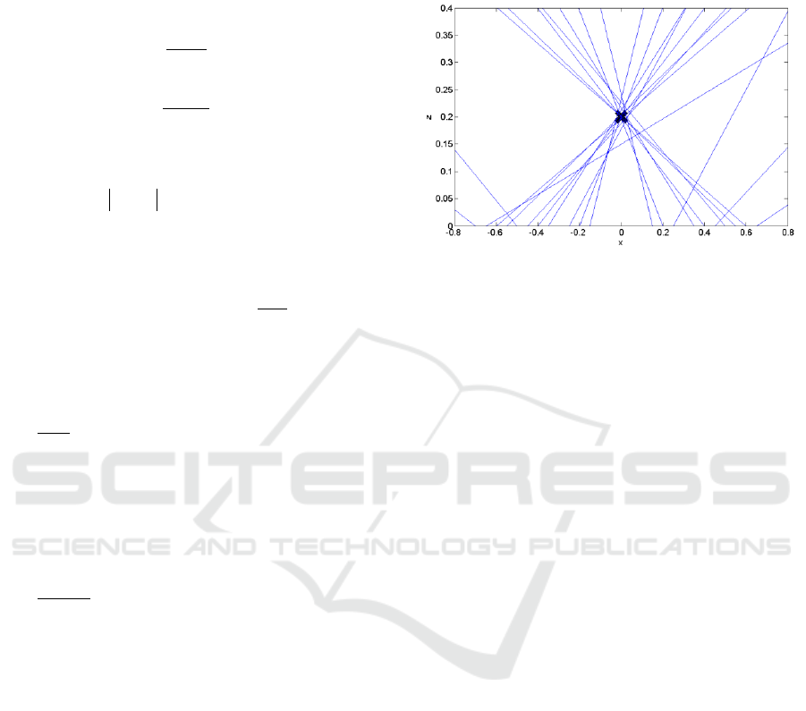
illustrated in the Fig. 1.
In this example, the array consists of 31 sensors
that give us 29 estimates of angles. Here the black
cross in the center illustrates the source position.
There are some missed rays at the picture that means
that it was impossible to estimate a frequency by the
considered algorithm and some beams are pointed
far away from the true source position. These facts
can be explained by failures and errors of the
estimation algorithm due to noise action.
Figure 1: Plot of estimated local directions of arrival for
the source located at the boresight.
If we look at the points of rays crossing, we can
see that the spatial distribution of them is torn with
multiple outliers, but the biggest density is around
the true source position. To find the source position
the distribution peak position must be estimated as
median of all crossing points coordinates.
3 SIMULATION RESULTS
The effectiveness of two proposed approaches was
analyzed and the far-field algorithm additionally
compared to the ML single-tone estimator and
Cramer-Rao lower bound (Rife, Boorstyn, 1974).
Statistical simulations by the Monte-Carlo
approach were done under the next conditions:
number of sensors in the ULA for a far-field case
N=11, for near-field N=31; due to limited range of
the used estimation algorithm, sensors spacing
distance is
4/
c
d 
; number of independent runs
with single-shot measurements for each plot is 1000.
The first experiments (Fig. 2) represent
performance of methods for different directions of
arrival under signal-to-noise ratio SNR=20 dB.
One can see that proposed approach works pretty
well in the range 0.2–1.4 rad. On the other hand its
performance decreases when source is located at
boresight or endfire positions because they
corresponds to boundaries of the estimation range.
Figure 3 shows performance for different SNR at
direction of arrival
 45
. One can see, that the
proposed method almost reaches the ML-estimator,
especially at high SNR.
Fourth International Conference on Telecommunications and Remote Sensing
56

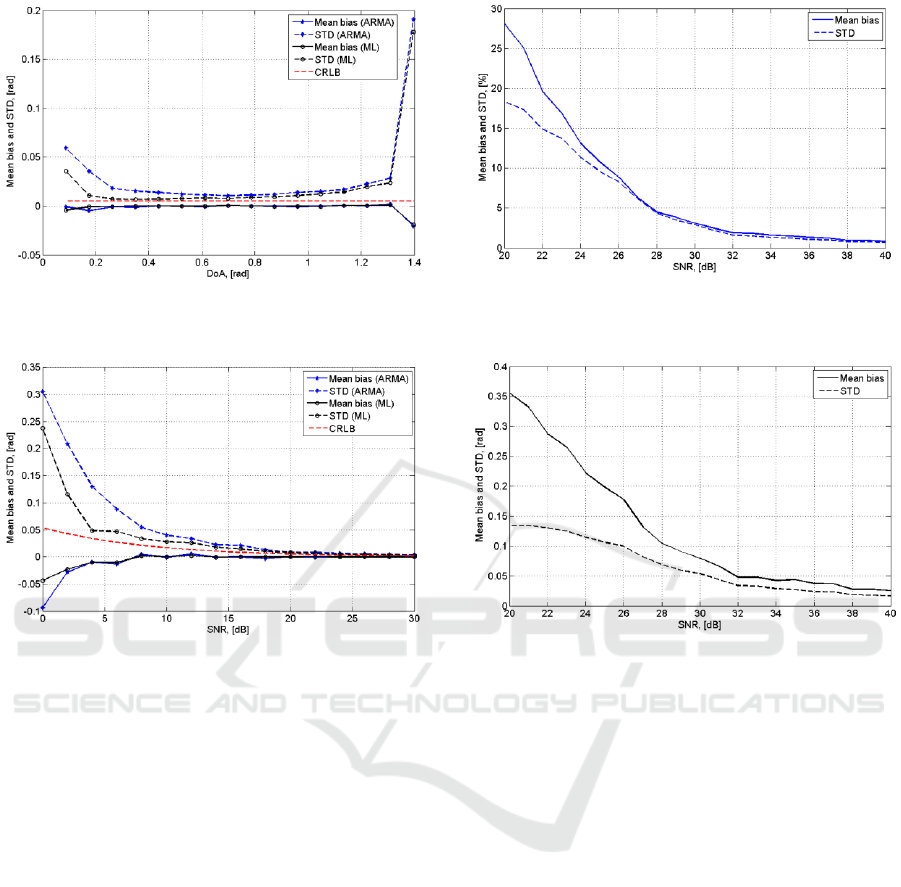
Figure 2: Dependence of the DOA estimation precision of
far-field algorithms on the its value.
Figure 3: Dependence of the DOA estimation precision of
far-field algorithms on the SNR.
The near-field estimation algorithm was analysed
under the SNR=20 dB for the source located
c
2
forward and
c
2
right from the beginning of the
ULA. The signal was simulated as a real part of the
model (Bai et al., 2013, p. 15). Figures 4 and 5
shows precision indicators for the range and the
DOA. One can see, that the proposed approach
requires quite high SNR (>30 dB) for decent
estimation quality, even with comparatively big
number of sensors. This can be explained by the fact
that local spatial frequency is estimated only in 3-
point running window and under this condition the
algorithm is pretty sensitive to the noise action. On
the bigger distance to the source using of bigger
windows becomes possible and precision increases.
Figure 4: Dependence of the range estimation precision of
the near-field algorithm on the SNR.
Figure 5: Dependence of the DOA estimation precision of
the near-field algorithm on the SNR.
4 CONCLUSIONS
The proposed far-field method shows performance
close to the maximum likelihood estimator in the
range between boresight and endfire source
positions, when SNR is bigger than 5 dB for few
sensors. The near-field method generally requires
bigger amount of sensors in comparison to far-field
method and gives relatively unbiased estimates only
at SNR higher than 30 dB.
ACKNOWLEDGEMENTS
The research work reported in the paper was partly
supported by the Project AComIn "Advanced
Computing for Innovation"; grant 316087, funded
by the FP7 Capacity Programme.
Fast Direction-of-Arrival Estimation for Single Source
Near- and Far-Field Approaches for 1D Source Localization
57

REFERENCES
Bai, R. M., Ih, J. G., and Benesty, J. (2013). Acoustic
Array Systems. Singapore: John Wiley & Sons
Singapore Pte. Ltd.
Chen, C. E., Lorenzelli, F., Hudson, R. E., and Yao, K.
(2008). Stochastic maximum-likelihood DOA
estimation in the presence of unknown non-uniform
noise. IEEE Int. Conf. on Acoustics, Speech and
Signal Processing (Las Vegas, USA, March 31 -April
4 2008), ICASSP 2008, 2481–2484.
Gao, F., Gershman, A. B. (2005). A Generalized ESPRIT
Approach to Direction-of-Arrival Estimation. IEEE
Signal Process. Letters, 12 (3), 254–257.
Grosicki, E., Abed-Meraim, K., and Hua, Y. (2005). A
weighted linear prediction method for near-field
source localization. IEEE Trans. on Signal Process.,
53, 3651–3660.
Johnson, R. C. (2006). Antenna Engineering Handbook
(3rd ed.). McGraw-Hill, Inc.
Prokopenko, I. G., Omelchuk, I. P., and Chyrka, Y. D.
(2012). Robust frequency estimation. International
Radar Symposium (Warsaw, Poland, May 23–25),
IRS–2012, 319–321.
Rife D. C., Boorstyn, R. R. (1974). Single-tone parameter
estimation from discrete-time observations. IEEE:
Trans. on information theory. 5, 591–598.
Stoica, P. and Besson, O. (2000). Maximum likelihood
DOA estimation for constant-modulus signal. IEEE
Electronics Letters, 36(9), 849–851.
Stoica, P., and Nehorai, A. (1989). MUSIC, Maximum
Likelihood, and Cramer-Rao Bound. IEEE Trans. on
Acoustics and Signal Process., 37 (5), 720–741.
Swindlehurst A. L., and Kailath T. (1988). Passive
direction of arrival and range estimation for near-field
sources. IEEE Spec. Est. and Mod. Workshop, 123–
128.
Wax, M. (1982) Detection and estimation of superimposed
signals, Ph. D. Dissertation, Stanford University.
Wu, Y., Liu, H., and So, H. C. (2009) Fast and accurate
direction-of-arrival estimation for a single source.
Progress In Electromagnetics Research C, 6, 13–20.
Yang, D., Shi, J., Liu, B. (2009) DOA Estimation for the
Near-field Correlated Sources with Interpolated Array
Technique. 4th IEEE Conference on Industrial
Electronics and Applications (Xi’an, China, 25–27
May 2009), ICIEA 2009, 3011–3015.
Zhi, W., and Chia, M. Y-W. (2007). Near-field source
localization via symmetric subarrays. IEEE Signal
Process. Letters, 14(6), 409–412.
Fourth International Conference on Telecommunications and Remote Sensing
58